Hello, dear friend, you can consult us at any time if you have any questions, add WeChat: daixieit

Computational Data Analysis for Ocean and Earth Scientists

SOES3042/6025 – Assignment 2 (Signal)

In this assignment, you will apply the signal theory learned in the lectures and the programming skills gained from the practicals to analyse real-world data in much the same way as you would for a genuine research project. You will encounter difficulties that are common when dealing with real-world data, and you will use your initiative to address them. You will look at two oceanographic data sets obtained via remote sensing: one physical data set (sea surface height anomaly) and one biological data set (surface chlorophyll concentration). You will apply signal-processing methods to extract information from each dataset and relate them to one another.

Instructions

This assignment accounts for 60% of the overall module mark. You will need to submit two files via Turnitin by 2 pm, Monday 15^th December: (1) a PDF file reporting your answers (supported by relevant figures) to the problems and (2) a Jupyter Notebook file containing all the Python code you used to generate the answers and relevant figures. Name the files as “SOES3042_A2_ID_LastName.pdf” and “SOES3042_A2_ID_LastName.ipynb”, respectively. Replace “ID” with your 8-digit student ID and “LastName” with your last name. If you are taking SOES6025, replace “3042” with “6025”.

Please note that only the PDF file will be marked. Your code file will not be marked, but it is required and will enable me to see where your results came from. Use a separate code cell for each problem, ensuring that running the code cell will produce the corresponding results and plots shown in your report.   Complete this assignment following the instructions below.

(1) Write your answer in the form of an individual written and well-structured short report accompanied by suitable figures, using the Word answer template provided. Once you complete your answers for the assignment, please make sure you save your final answers as a PDF file and submit it via Turnitin. Please also:

§ Ensure that each task is clearly addressed and that you also describe your approach to the task (do this without referring to programming details).

§ Do more than simply produce figures and answers to the direct questions. Ask yourself and try to provide answers to questions like: What approximations or assumptions have I made in answering this point? Can I justify these? How do I expect them to affect my results? Is there a way to verify this expectation (the answer may be no)? High marks will only be awarded to answers showing evidence of this thought process.

(2) While using the answer template, you may adjust the size of the answer boxes of “short report” and “figures” for each problem (i.e., Problem 1, Problem 2, etc.), but make sure the answer for each Problem (with “short report” and “figures” combined) does not exceed one side of an A4 paper. Start the answer for a new Problem (i.e., Problem 2, Problem 3, etc.) on a new page. Please use single-line spacing and a font size no smaller than 11 pt.

The data sets

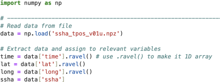
This assignment is associated with two data sets: ssha_tpos_v01u.npz and chlo_swtp_v20b.npz. As you learned from the first part of the module, you can read these .npz files using the load() function in NumPy and then extract relevant data. For example, the following code will allow you to extract the time, lat, long, and ssha data.

Relevant information about the two data sets is provided in the table below.

Thanks to Paolo Cipollini for providing the data for this assignment and to Florian Sévellec, Kevin Oliver, and Simon Müller for participating in the design of this assignment. The data sets are not to be copied and used for any purpose other than this analysis exercise.

The assignment

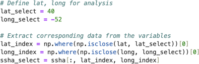
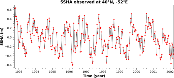
Load the SSHA data for the mid-latitude North Atlantic from file ssha_tpos_v01u.npz. Make sure you understand the data (referring to the table above), how they are organised, and that your code can extract data from different locations properly. As an exercise, reproduce the plot below that shows SSHA as a function of time at the location: 40°N, 52°W. The following code utilising the where() (which you used in Practicals 3 & 4 ) and the isclose() functions in NumPy should get you started.

Problem 1 (25 points for SOES3042, 20 points for SOES6025): Determine the amplitude of the annual cycle in the SSHA data at 39°N, 58°W using the Fast Fourier Transform. Include a frequency versus amplitude plot in your report and annotate the frequency and amplitude values for the annual frequency on the plot.

Hint: You probably want to make clear the procedures you followed to check for and fix potential issues associated with your analysis (e.g., is the time series evenly spaced? Is there a trend? Is sampling/aliasing a problem? Could spectral leakage happen? etc.). Also, pay attention to the order these checks/fixes should happen.

Problem 2 (25 points for SOES3042, 20 points for SOES6025): Filter the data at 39°N, 58°W to produce two new time series: one showing the annual cycle only, and the other showing the signal with the annual cycle and higher frequencies removed.

Include information on how you constructed your filters and how you applied them etc. Include comparison plots of the original and filtered spectra in the frequency domain, and comparison plots of original and filtered signals in the time domain.

Problem 3 (25 points for SOES3042, 20 points for SOES6025): Create two maps: one showing the amplitude of the annual cycle in the SSHA data at all available locations in the region from 0°W–80°W in longitude and from 25°N–45°N in latitude in the North Atlantic, and the other showing the amplitude of the annual cycle in the log₁₀(chl) data within the same region (using the chlorophyll data set in the data file chlo_swtp_v20b.npz). The maps should be associated with appropriate colour scales. Include comments on issues you encountered processing the data and how you dealt with them.

Hint: To create such a map, you will need to apply a Fourier transform at each location, which could be achieved, for example, using a for-loop over longitude, nested inside a for-loop over latitude.

You will likely encounter difficulties associated with missing data. In some cases, this is due to the presence of land (hence, missing data for all time steps at these locations). But in other cases (especially for log₁₀(chl) data), only a small amount of data is missing at some time steps (e.g., because of cloud cover etc.). You need to find a way to analyse the data that do exist at those locations.

Problem 4 (25 points for SOES3042, 20 points for SOES6025): You will notice that at around 36°N, 55°W, the annual frequency amplitude signal is large in both the SSHA and the log₁₀(chl) data. Extract SSHA data from 36°N, 55°W, and log₁₀(chl) data from 36.25°N, 55.25°W, then estimate the lag (in unit of months) between SSHA and log₁₀(chl) data at the annual frequency using cross-correlation and cross-spectral analyses of the two time series.

Make clear of the steps involved in the process. The report should include the following plots: direct comparison of the two time series over the common time axis, the normalised cross-correlation between the two time series, frequency vs the cross-spectrum magnitude, and frequency vs the phase associated with the cross-spectral analysis.

Problem 5 (20 points for SOES6025 only): Determine the spatial variation of the lag at the annual frequency between the SSHA data and the log₁₀(chl) data by creating a map of the lag in the region of  0°W–80°W in longitude and 25°N–45°N in latitude. 

Hint: You should have noticed that the lat and long grids and the time range and steps are not the same for the SSHA and the log₁₀(chl) data. You can use 3D interpolation to interpolate both datasets onto the same time, lat, and long grids. This can be achieved using RegularGridInterpolator in SciPy (e.g., from scipy.interpolate import RegularGridInterpolator). See descriptions about and examples of using RegularGridInterpolator here. 

When the two datasets are on the same time, lat, and long grids, to create a lag map (for the annual frequency), you will need to repeat the lag estimation (as you did for Problem 4) at each location in the selected latitude and longitude range. Similar to Problem 3, this could be achieved, for example, using a for-loop over longitude, nested inside a for-loop over latitude. Note that you may still encounter missing data issues at some locations (similar to Problem 3) and you will need to find a way to analyse the data that do exist at those locations.