Hello, dear friend, you can consult us at any time if you have any questions, add WeChat: daixieit

Excel Funds and Apps

Lab session

Module 3

All those exercises must be completed and submitted in the corresponding dropbox on K2

Exercise 1

You will find on K2 a file named « Exercise1”. This Excel document contains many different worksheets. You must complete the different worksheet by adding formulas, pivot table, charts and by setting the presentation according to the specification found below:

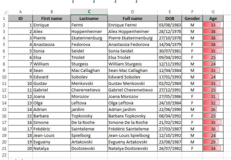
Worksheet “Directors”:

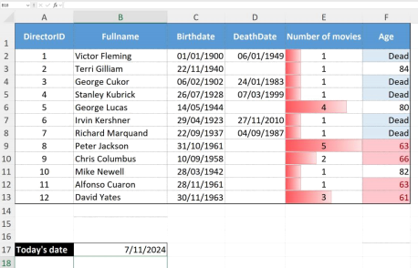
In this worksheet you must do the following work:

Work to be done

Format the column C and D as dates

Add a formula in the range E2:E13 in order to count the number of movies for each director. You must count in the column D in the worksheet “Movies” the number of cells with a value equal to the directorID found in the column A in this worksheet.

The formula that you must insert in the range from F2 to F13 will display “Dead” in the cell if the DeathDate is not empty (ISBLANCK()). Else it will calculate the age by (using the today’s date found in the cell A17 and the birth date in column C). Manage to display the values in the cells without any decimal positions. This formula will subtract the birthdate from today’s date and divide this by 365.

Set a dark blue shading for the cells on the first line, set the text in those cells in bold and white

Add an external thick border around the table and dotted lines for the inner border

Center column 1 (A2 to A13) and column 5 (E2 to E13)

Align Column 3 (C2:C13),4 (D2:D13) and 6 (F2:F13) to the right and center vertically

Center the first line both horizontally and vertically

Adjust the width of the columns to the content (in order to make everything visible)

Add a conditional format to the column E (from line 2 to 13) in order to display red “Data bars” whose size are calculated according to the value found in the cells.

Add a conditional format to the last column in order to set a light blue background for the cells that contain the value “Dead” and another conditional format in order to highlight with a pink background and a red text all the cells with a value less than the average.

Manage to have all the cells on the first row centered horizontally and vertically.

Set a black background and a white bold text for cell A17.

The cell B17 must be displayed as a short date. The cells A17 and B17 must be surrounded by a thick black border.

Worksheet « Movies »:

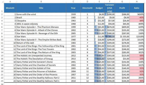
Work to be done

Add in the column G from line 2 to 23 a formula that calculate the profit by doing a subtraction between the value found in column F and E.

Add in column H from line 2 to 23 a formula in order to calculate the ratio between the profit and the budget (column E). You must divide the profit by the budget and display the result as a percentage with no decimal positions.

Format the column E, F and G as currency (using the $ as the currency symbol)

The first line (title line in row 1) must be automatically wrapped, centered horizontally and vertically

The first column (A2:A23) must be aligned to the right horizontally

The second column (B2:B23) must be aligned to the left

Columns C to D must be centered

Add a thick black border around the table, the inside lines must be black and dotted.

Set a dark blue shading for the cells on the first line, the text must be bold and white.

Add a conditional format to the last column to highlight using a pink background and a red text for all the cells with a value less than 100%.

Add a conditional format with blue gradient data bars to the column E and then do the same with column F.

All the cells in the table must be centered vertically

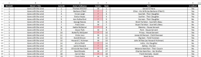
Worksheet « Actors »

Work to be done

Add in column D (Number of movies) a formula that counts in the worksheet “Casts” the number of time each actor’s id can be found in column C.

• All the cells must be centered horizontally and vertically

• The first line must have a dark blue background

• The text on the first line must be white, bold and italic

• There must be a thick black border all around the table

• The inside border must be blue and dotted

• The last column (E) must use an accounting format with a currency symbol set to $

Add two conditional format to the last column in order to highlight with a pink background and a red text the top ten cells in this column and another one in order to highlight with a light blue background and a dark blue text the bottom ten percentcells in this column.

Work to be done

Add formulas in the cells I3 and I4 in order to count the number of women and men in the actors based on column C. Add a formula in the cell I5 to do the sum of the cells I3 and I4.

Add a formula in the cell I9 that can be propagated to cell I10 in order to calculate in cell I9 the ratio between the number of women and the total number of actors and in cell I10 the ratio between the number of male actors and the total number of actors (two divisions)

Add formulas in the cells from I14 to I17 in order to calculate the min, max, average and standard deviation of the cost per day.

Format the tables in order to make it look like the model above:

• The first line for the three tables must be merged and centered

• This first line for each table must have a dark blue background and a bold and white text

• The left column must be right-aligned and have a bold text

• The right column must be aligned to the left.

• The values in the range I14:I17 must use an accounting format with a $ symbol.

Worksheet “Casts”

Work to be done

Add in column B a formula using a vlookup in order to retrieve the movie’s title (from the worksheet “Movies”) based on the MovieID found in the adjacent column to the left..

Add in column D a formula to retrieve the actor’s fullname from the worksheet depending on the ActorID found in the adjacent column to the left.

Add in column E a formula to retrieve the gender from the worksheet depending on the ActorID found in the column C.

Manage to format the table as shown in the above model.

• All the border must be visible using a solid black thin line

• The first line must have a black background and a white and bold text

• All the cells must be centered horizontally and vertically

• Add a conditional format on the column E to highlight with a pink background and a red text all the cells containing “F”

• Adjust the width of all the columns

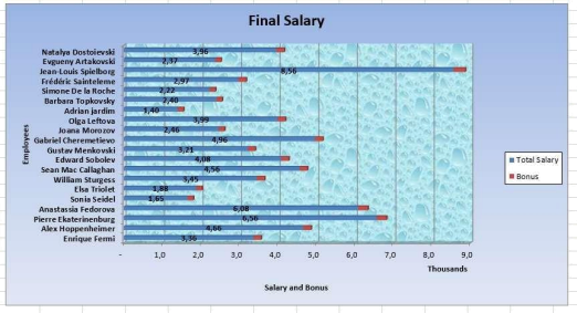
Worksheet « Charts »

Work to be done

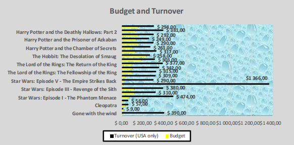
Build from the worksheet « Movies » a Bar chart that displays the “Budget” and “Turnover”.

Make it look exactly like the one above

1. The bars of the turnover must be black

2. The bars for the buget must be yellow

3. X axis labels visible (using the movies’ titles)

4. Droplet Texture for the plot area

5. Grey background for the chart

6. The legend must be visible to the bottom and formatted as shown above.

7. The title of the chart must be visible above the Plot area as shown in the model

8. The data labels must be visible for the turnover only.

Exercise 2

You will find on K2 a file named « Exercise2.xlsx» that will be used for this excel part. It contains many different worksheets.

In this worksheet you must do the following work:

Work to be done Worksheet “Part 1”

Add a formula in the range D2:D21 that builds the full name by “adding” the last and first name.

Add a formula in the range G2:G21 that calculates the age for the sellers (using the today’s date found in the cell A23 and the birth date in column E). Manage to display the values in the cells without any decimal positions

Set a grey shading for the cells on the first line, set the text in those cells in bold

Set text align to the center and center vertically

Add all the borders for the table

Align columns 1 and 5 (Columns A and E) to the right and center vertically

Align Column 2,3,4 (Columns B,C,D) to the left and center vertically

Center columns 6 and 7 (Columns F,G) and center vertically

Center the first line both horizontally and vertically

Format the column E as a date

Adjust the width of the columns to the content (in order to make everything visible)

Add a conditional format to the last column in order to display red “Data bars” whose size are calculated according to the value found in the cells.

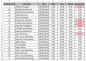
Work to be done worksheet “Part 2”

Add in column B a formula that retrieves from the table in worksheet “Part 1” the full name for the customer.

Add in the last column a formula in order to calculate the work time (using the start time in column D, the end time incolumn E and the break time in column F). You will subtract the start and break times to the end date.

Format the column C as a short date

Format columns D:G as Time

The first column must be centered horizontally

The second column must be aligned to the left

Columns C to G must be centered

Add all the borders

Set a grey shading for the cells on the first line

Add a conditional format to the last column to display the five top values

The text in cells on the first line must be bold and centered horizontally

Sort entries from newest to oldest with respect to Column “Day”

All the cells in the table must be centered vertically

Part 3

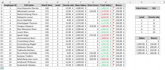
Work to be done

Add in the range E1:E21 a formula that retrieves the value of the hourly rate depending on the value found in the column D and the table in the range K5 to L10.

Add in the range F2:F21 a formula that calculates the “Base Salary” by multiplying the hourly rate (column E) with the work time in column C.

Add in the range G2:G21 a formula that calculates the extra hours (if any) by calculating the difference between the work time and the value found in the cell L2. This difference if positive must then be multiplied by the “hourly rate” (column E) else the value must be replaced by a zero.

Add in the range H2:H21 a formula that calculates the sum of the “base salary” and the “extra hours”.

Add in the range I2:I21 a formula that retrieves the bonus from the table K12:L17 (You must type the data in your excel document based on what you see in the model above) base on the calculated Total salary.

Set the presentation according to the following instructions

• The first line of all the tables and the cell K2 must have a grey background and a black and bold text.

• All the border must be visible for all the tables in this worksheet

• The cells in the ranges E2:I 21 (Hourly rate:Bonus) and K13:L17 (Salary table) must use an accounting format and must be aligned to the right.

• The columns A, C and D, the ranges K6:L10 and K13:L17 must be centered.

• All the cells must be entered vertically.

• There must be an icon set in the column I (use the same as the one you can see in the model above)

Add two conditional formats to the “Total Salary” column in order to highlight in red the values above the average and in green the values below the average.

Part 4

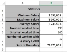
Work to be done

Add formula in cell B2 to find the minimum value in the column H (in “Part 4”)

Add formula in cell B3 to find the maximum value in the column H (in “Part 4”)

Add formula in cell B4 to calculate the average of the values in the column H (in “Part 4”)

Add formula in cell B5 to find the greatest worked time from column C (in “Part 4”)

Add formula in cell B6 to find the smallest worked time from column C (in “Part 4”)

Add formula in cell B7 to count the number of workers with a value in column H greater than 2000 (in “Part 4”)

Add formula in cell B7 to calculate the sum of the salary for workers in column H (in “Part 4”)

You must set the presentation according to the model (including the merged cells and the wrapped text).

Part 5

Work to be done

Build from the worksheet « Part 3 » a stacked 3D bar chart that displays the “Total salary” and the “Bonus”.

Display the chart in worksheet “Part 5”.

Make it look exactly like the one above according to the instructions below:

• The legend must be visible to the right.

• The data labels must be visible and bold.

• The X axis labels must be the full name of the employee.

• The display unit for the Y axis must be “Thousands”.

• The wall of the chart must use the texture you can see in the model.

• The chart must have a blue gradient filling.

• The title of the chart must be visible and bold.

• The X and Y axis title must be visible with the text you see in the model.

Exercise 3

The file « Exercise3.xlsx » contains a workbook with five worksheets.

• The worksheet “Customers” contains the full list of our customers.

• The worksheet “Products” contains the full list of all the products we’re selling.

• The worksheet “Orders” contains the full list of all the orders. Each one is associated with a customer through the column “CustomerID”.

• The worksheet “Order’s Products List” contains the details of the orders. Each line in this worksheet is associated with an order through the column “OrderID”. The column “ProductId” tells us which product was ordered.

• The last worksheet “Discount - Shipping” contains a table that tells us the discount to be granted based on the amount of the orders (it already has the name “Discounts”). There is also a second table that provides the shipping cost for each zipcode (this one is already named “Shipping”).

In the worksheet “ Order’s products list ”:

• You must provide in the column “Product name” a formula (using a vlookup) that will retrieve from the table products the “Product’s name” base on the ProductID.

• You must do the same to get the “Price per Unit”.

• You must calculate the “Amount” of the orders by multiplying the “Quantity” with the “Price per Unit”.

The worksheet “Orders” must also be completed by providing formulas for the last five columns.

• The first column to be completed is the column “Amount”. This column must contain a formula that will use a sumif to get the sum of the amount for all the related lines in the worksheet “Order’s products list”.

• The second column “Discount to be granted” will use an approximate vlookup to get the discount that must be granted based on the amount of the order.

• The third one will get using a vlookup the shipping cost for this order depending on the Zipcode for the associated Customer (to get that information you will use a vlookup).

• The fourth column will calculate the “Final Price” by adding the shipping cost and subtracting the discount to the value of the column “Amount”.

• The fifth one will use a countif to calculate the number of products for this order (i.e., the number of row having the same OrderID in the worksheet “Order’s products list”.

The worksheet “Products” must be completed by providing three formula in the last three columns:

• The column “Total Turnover” must contain the sum of the amount for all the lines in the worksheet “Order’s products list” that are having the same ProductID.

• The column Number of Orders will contain a formula to count the number of rows in the worksheet “Order’s products list” that are having the same ProductID (using a countif and assuming no one will have bought the same product twice in the same order).

• The column “Total number of units sold” will use a sumif to do the sum of the column “Quantity” for all the rows having the same ProductID in the worksheet “Order’s products list”.

The worksheet “Customers” must be completed by providing two formulas for the last two columns:

• The column Number of orders will count how many rows are related to this customer in the worksheet “Orders”.

• The column “Customer’s turnover” will be calculated by doing the sum of the column “final price” from the worksheet “Orders” (assuming only the rows for which the CustomerID matches one of the Customers we’re writing the formula for).

You must add a conditional format to highlight all the zero values in the column “Customer’s turnover” in the worksheet Customers. The second format we will set will allow us to highlight all the cells containing a zero value in the worksheet “Products”.

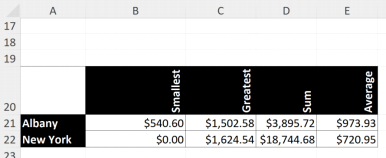
Finally we want to add a new worksheet that we will name “Cities” and in which we want to calculate some statistical quantities related to those cities. (You can get all cities by using function UNIQUE())

Your table will look like this:

Finally, you must provide in this same worksheet a few formulas to determine the smallest, greatest, the sum and average of the amount for the column “Customer’s turnover” for customers living in “Albany” and “New York”. Your answers should like this: