This paper contains FIVE questions, and each question is worth 25 marks.

Answer FOUR questions in total.

If you attempt more questions than required, only the required          number of answers will be marked. Please strike through any           answers that you do not wish to be marked. If you do not do this the marker will mark the answers in the order that they appear in your    exam booklet(s).

For each question, an outline marking scheme is shown in brackets to the right of each question.

Only University approved calculators may be used.

A foreign language direct ‘Word to Word’ translation dictionary (paper version) ONLY is permitted provided it contains no notes, additions or annotations.

1.     Provide a brief explanation of the following:

a)   homoscedasticity

[5 marks]

b)   moving average (MA) model

[5 marks]

c)    kurtosis

[5 marks]

d)   non-rejection region

[5 marks]

e)   the F-test

[5 marks]

2.     Suppose that two variables,  and  , are related by means of the following regression model:    =  +  . Notice there is no constant in the regression, a special case of the regression line.

a)   Assuming this  is  a  good  description of the  relationship between  the  two  variables,  find  ,  the  Ordinary  Least Squares (OLS) estimator of  .

[10 marks]

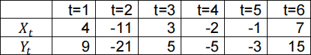
b)   Using the sample of six observations below, compute:

i)       , the OLS estimator of  obtained in a).

ii)    the sample estimator of the variance of the error term Var().

 [7 marks]

c)    Explain any two properties of the OLS estimator.

[8 marks]

A3.  This exercise is based on the CAPM model, as well as the

Fama and French three factor and the four factor models. Three regressions were estimated, and the most relevant output has been summarised in the following table:

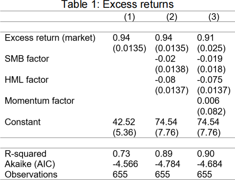
Notes: The coefficients are estimated by OLS; their standard errors are in parentheses.

The dependent variable is the excess return on a portfolio of 50 stocks over the risk-free interest rate. The free risk asset to compute excess of return is the 3-month treasury bill.

a)   In  column  (1), the  regression  includes only the  excess returns on the market (proxied by the stock market index). Explain how this regression tests the CAPM model and the meaning of the two coefficients.

[7 marks]

b)   In column (2), two additional factors are considered: the book-to-market factor (HML) and the size factor (SMB). This is the three-factor model. Does this model fit the data better than the CAPM? Perform the suitable hypothesis test to support your answer.

[7 marks]

c)    In column  (3), we consider one additional factor to the previous model. This is the so-called “momentum” factor, which captures the tendency for the stock price to continue rising if it is going up and to continue declining if it is going down.  Should the  momentum factor  be  included  in the regression? Perform the suitable hypothesis test to support your answer.

[5 marks]

d) The  table  also  indicates  the  R-squared  and  the  Akaike information criterion for each of the three regressions. Using these statistics, which model would you select as the best?

[6 marks]

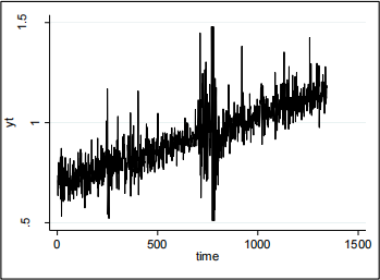
4.     The main variable of interest is yt.

a)   Use the Stata output below to test if the variable features a unit root. What is the conclusion?

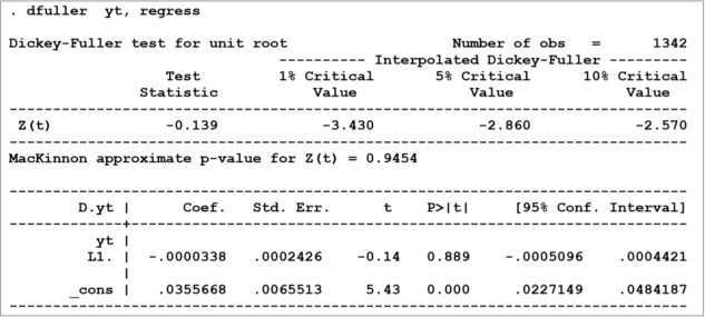
[9 marks]

b)   We now perform a second test, adding a time trend to the model outlined in part a). Below you can find the Stata

output. Perform the test for a unit root. Is the conclusion the same than in a)? Explain the differences between the two tests.

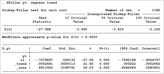
[9 marks]

c)    Below you can find a plot of the series  over the relevant time period. What does this plot suggest regarding the two tests for a unit root you have carried out?

[7 marks]

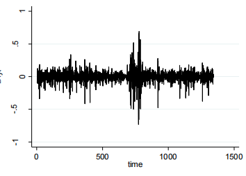
5.     The  exchange  rate  in  logs  is  represented  by  ,  which  is measured with a daily frequency. The main variable of interest is its first difference (∆).

a)   The plot below shows ∆ over time. Explain the concept of volatility clustering.

[8 marks]

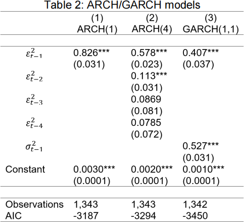
b) The table below shows estimates of three models of volatility: ARCH(1), ARCH(4) and GARCH(1,1). In the three models,  the  conditional  mean  equation  for ∆  only  includes  an  intercept  ( ∆ =  +  ,  where   is  the  error  term  with  variance 2).

i)    Outline the equation for the conditional variance of the ARCH(1)  model.  Based on  column  (1),  identify the estimates of the key parameters.

[7 marks]

ii)    Explain which of the three models provides the best fit and compare them.