CS 1100 – Computer Science and Its Applications Topic 3
Hello, dear friend, you can consult us at any time if you have any questions, add WeChat: daixieit
CS 1100 — Computer Science and Its Applications
Topic 3: Using More Advanced Functions
How to Get Started
To get started, download the starter file from Canvas. The link is close to the link where you got these assignment instructions.
What to Turn in
You must submit your solution to Canvas by the due date. You will be creating a spreadsheet using either Microsoft Excel or Google Sheets. When you finish the assignment, save the file and upload it to Canvas. You must name the file
LastName-FirstName .advanced-fns
where LastName is your last name and FirstName is your full first name.
Saving the file
You save the file using the Save as. . . command of the File tab.
You should also turn on the Auto-save option in the top left corner of the window to make sure you do not lose any data.
How to Create a Shareable Link for Your Claude Conversation
For some problems, you turn in your chats to demonstrate your prompting skills for using Claude as a personal tutor to learn about spreadsheet technology (primarily Excel but also Google Sheets). We will give you feedback on your chats. We use links to your chats at OpenAI to read them.
1. Step 1: Prepare a New Worksheet
In the same Excel submission file, create a new worksheet named "Claude." Create a table with two columns:
• The first column should contain the name of the problem (e.g., T2 Problem 2 Subproblem 5).
• The second column should contain the Claude shareable link.
2. Step 2: Create a Shareable Link for Claude
Open your Claude conversation in the left window, and follow these steps:
(a) Click on the top-right sharing widget. Make sure you create a link that is shared with anyone in NU (which includes your TA and professor).
(b) Select "Copy Link" and paste it into the newly created worksheet in Step 1.
Because you use expensive Claude technology, you might be interested in how it works at a high level of abstraction. The following entertaining talk gives you a useful background. https://www.youtube.com/ watch?v=_6R7Ym6Vy_I
Knowledge Needed
This assignment involves the following Excel functions and techniques:
• EDATE() (or DATE()), SEQUENCE(), DATEDIF(), QUOTIENT(), SUM(), MOD(), TRUNC(), COUNTA(), PMT(), LAMBDA(), LET.
• What-if analysis using dynamic array formulas.
• Formatting
Keep in mind that how you express the formulas matters and is part of the grading. It’s not just getting the right answer that counts; how you write the formulas matters too. Use good naming for intermediate results and develop your LAMBDA formulas incrementally using the LET function.
Note: Please note the rubric shown in Canvas that gives you detailed information about how points are assigned to your solutions.
Problem 1 Collecting Interest (43 points: 10 for chats)
There’s an urban legend that Albert Einstein once said compound interest is the most powerful force in the universe. While this attribution is not substantiated, he did apparently say
“Compound interest is the eighth wonder of the world. He who understands it, earns it. . . he who doesn’t. . . pays it.”
The basic formula for compound interest (without regular and extra deposits) is
A = P * (1 + r /n)n*t
where P is the starting balance, r is the annual interest rate, n is the number of times interest is com- pounded per year and t is the number of years.
The worksheet Savings Interest represents a savings account calculator. Use name ranges in formulas where appropriate. Deposits are made monthly. The monthly interest rate equals to the annual interest rate divided by 12.
Another note: the starting date uses TODAY() by default. TODAY() returns the current date.
You can use the FORMULATEXT() function to display the formulas near the columns where they have been used.
There is a cell labelled "months to try", which you can use to experiment with the problem with a set number of months.
The first 5 columns (DepNo. -> Total Deposits) are expected to be array formulas which are spillable.
The rest of the columns should have draggable formulas unless you know how to automate the iteration.
Put your responses into the worksheet Savings Interest.
1. (1 pt) Create named ranges for each input (D6:D12) and for H12.
2. (1 pt) Our planning goal will be to double our savings. D12 will be twice the starting balance.
3. (23 pts) There are 9 columns, each worth 1 point, except Deposit Date is worth 5 points and Extra Deposit is worth 9 points. Use formulas to fill in the columns, including the column for DepNo. We’re going to assume the deposits go in at the first of the month, which means the interest accrued will be for the entire balance, the starting balance plus the new deposits. Let’s group the two deposits (scheduled or extra) together as:
Total deposits = scheduled deposit + extra deposit
The formula to calculate the balance at the end of the month is:
ending Balance = beginning balance + Total deposits +
(month’s beginning balance + deposits) × interest rate
(a) Use EDATE() or DATE() to fill in the Deposit Date column.
Write a LAMBDA formula which takes 3 arguments date, n, k, where date is a date (e.g., TODAY() or DATE(2022,1,1)), n is the number of dates produced and k indicates how many months apart the dates must be. Your LAMBDA formula starts like this LAMBDA(date,n,k,...) and it will use somewhere the SEQUENCE function. Use your LAMBDA formula to compute the deposit dates in your savings account calculator.
EDATE(given date, months) adds months to a date. It calculates a date k months after a given date. For example, EDATE(“1/1/2020”, 5) returns “6/1/2020.”
You can also use the DATE() function. To go this route, you need to pass three parameters, each of which uses a function: YEAR(), MONTH(), and DAY(). You would enter the year, month, and day into each function. Suppose we have a date in B3, to find the date a month from B3, you would write =DATE(YEAR(B3), MONTH(B3) + 1, DAY(B3)) .
Consider the following partial solution.
=LAMBDA(date,n,k,
LET(
indices, SEQUENCE(n, 1, 0, 1),
months_to_add, MAP(indices, LAMBDA(i,UNKNOWN_1)),
result, MAP(months_to_add, LAMBDA(m, UNKNOWN_2)),
result
)
)
Turn in the completed solution by assigning to each UNKNOWN an Excel formula, for example, a function call or an arithmetic expression.
Use Claude to assist you in solving the problem and turn in the chat. Ask Claude to give you hints to answer this problem using two approaches. First, solve the problem with dragging (creating many formulas,) and then solve it with one formula starting with LAMBDA. Claude will speed up your solution process and help you understand how the solution works. But be alert regarding errors you might get in the hints or explanations! Excel 365 will help you to identify them when you check Claude’s answer step by step. If Excel 365 gives an error message when you implement Claude’s hints or suggestions tell Claude about the error message or an erroneous output or your intuition of what might be wrong. Ask for an improved hint or suggestion.
If you don’t understand Claude’s hints, ask it for clarification. Turn in your sequence of prompts that lead to the successful hints.
(b) If you plan to put something extra in every month, D9 would be 1. For something extra every other month, D9 would be 2.
To compute the extra deposits write a LAMBDA formula LAMBDA(n,k,v,...), where n, k are positive integers,and v is a positive number (a floating point number). Produce a column of n cells so that every k-th cell contains value v and the other cells contain 0. The first cell is number 1. Use your LAMBDA formula to compute the extra deposits in your savings calculator. Remark: If you know the IF function, use it. If you don’t, use the property that TRUE*v=v and FALSE*v=0.
Use Claude to get hints on how to approach the problem and turn in the chat
Consider the following partial solution and correctly fill the UNKNOWNs:
=LAMBDA(n,k,v,
LET(
positions, UNKNOWN_1,
isKthPosition, LAMBDA(pos, MOD(pos, k) = 0),
depositValue, LAMBDA(pos, IF(isKthPosition(pos), v, 0)),
MAP(positions, UNKNOWN_2) ) )
4. (5 pts) In H6:H10 calculate a summary view.
5. (2 pts) Format the sheet to look similar to Figure 1.
6. (3 pts) Write a formula FV(...) that computes the ending balance of the savings account calculator after t months assuming that all extra deposits are 0. FV, one of the financial functions, calculates the future value of an investment based on a constant interest rate. As arguments to FV use formulas that involve the appropriately named cells from the top part of the savings account calculator.
7. (Bonus 2 pts) In H11, translate the number of months needed to reach the goal into a text string of y years and m months.
Key Considerations:
1. For DepNo., Deposit Date, Deposit, Extra Deposit, Total Deposit use only one formula which has months_to_try as parameter. Make sure your formulas for Beginning Balance, Interest etc., are “copyable” down, i.e., that they use named ranges or absolute references ($) wherever needed or appropriate.
2. Write formulas that are easy to read and understand by someone other than yourself.
Problem 2 Paying Interest (42 points: 10 for chats)
Having gained interest in Problem 1, now let’s look at its opposite, paying back a loan. In worksheet Paying Interest, you will determine how long it will take to pay off a loan. Loans have principal (the amount borrowed), an interest rate, a duration (the term), and a payment schedule (monthly, bi-weekly, etc.). The interest rate can greatly affect how much you pay back.
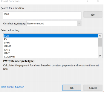
This problem uses a specialized function, PMT(), which calculates the monthly payment needed to pay back a loan on-time. It’s one of many built-in functions tuned to specific tasks. You should always look to see if there is a built-in function before you set about to do it by hand. Finding a function can be done in the ribbon.

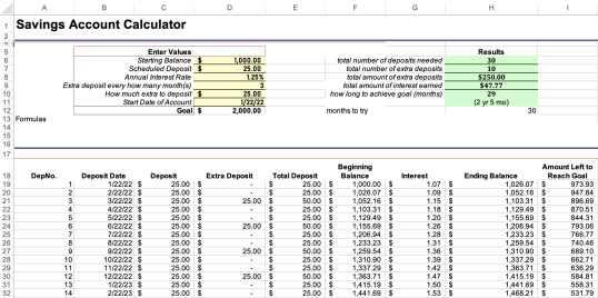
Figure 1: An example of what your sheet for Problem 1 should look like
Or, you can click on the fx button on the formula bar to raise the Insert Function dialogue box. If you look closely at the next example, you can see we didn’t know the function’s name, but instead looked for functions related to loans.
Objective: Determine the duration required to pay off a loan considering various interest rates and terms using a two-dimensional table.
Steps:
Set Up Input Fields:
Loan Amount: Input the principal amount. Interest Rate Range: Input the minimum and maximum possible interest rates. Interest Rate Column Headers:
Generate five evenly spaced interest rates between your minimum and maximum rates.
Objective: Determine the monthly payment required to pay off a loan considering various interest rates and terms using a two-dimensional table.
Steps:
1. Set Up Input Fields:
Loan Amount: Input the principal amount.
Interest Rate Range: Input the minimum and maximum possible interest rates.
2. Interest Rate Column Headers:
Generate five evenly spaced interest rates between your minimum and maximum rates.
Use a formula to compute these column headers automatically.
3. Yearly Term Row Headers:
List out terms from years 1 to 20.
4. Monthly Payment Calculation:
Position the formula in the upper-left corner of the table to compute monthly payments using the PMT() function.
Method 1: Drag the formula across the table.
Method 2: Use the dynamic array feature to spill the formula results throughout the table auto- matically.
Note: The lists of interest rates (horizontal) and terms (vertical) are to be generated using the SE- QUENCE function.
Implement the following steps. Use Claude to get hints to solve the problem and turn in the chat(s). Only ask for hints, not the final solution.
1. (4 pts) Create input fields for the amount loaned, the lowest possible interest rate, and the highest possible interest rate.
2. (4 pts) Create columns for looking at five interest rates evenly spaced between the lowest and highest input interest rates. This has to be done using a Formula to compute the column headers.
3. (6 pts) Use PMT() to calculate the monthly payment due if the loan of $50000 is paid in full at the end of the term. For instance, the monthly payment of a loan with a 4.75% interest rate given a five (5) year term is $937.85.
4. (2 pts) Format the model exactly as shown in Figure 2.
You may introduce intermediate calculations—and if you do, please do not hide them. Breaking complex calculations into smaller steps is a good idea. You can see our example calculated the step size for the interest rates in F1.
5. (7 pts) In the same sheet, create a table to summarize the total costs as shown in Figure 3. You should calculate the actual cost of the loan. From the Monthly Payment Due (MPD) table compute the Actual Cost (AC) table which gives for each interest rate and term the total amount of interest you paid over the duration of the loan. To compute AC, multiply each entry in MPD by the total number of periods and subtract the principal (Initial Balance).
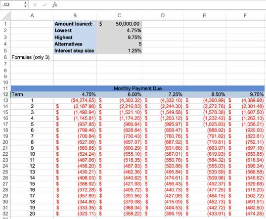
Figure 2: An example of what your payment sheet for Problem 2 should look like
6. (Bonus 2pts) Show two different ways of writing the formula in the upper left corner of the Actual Cost table. One is spilling and the other one needs to be copied. Indicate which of the two formulas requires copying to extend it to the entire table. Assume that the list of terms is defined using the SEQUENCE function. Assume that MPD is a two-dimensional named range covering the Monthly Payments Due table. You have a reference to the upper left corner of MPD to use in one of the two formulas. Discuss the advantages and disadvantages of the two formulas.
Problem 3 Writing your own MyMax function (15 points: 3 for chat)
Use Claude to get hints to solve the problem and turn in the chat. For this problem, create a new worksheet called MyMaxFunction. Write a function called MyMax(T), where T is a table of numbers. MyMax(T) returns the maximum number in T. You cannot use the Excel functions MAX, MAXA, or LARGE. But you have the built-in Excel function MIN available to define your implementation of MAX. Test your MyMax function with at least three inputs: a row with 4 numbers, a column with 4 numbers and a table of numbers with 4 rows and 2 columns. For example, one of your test cases might be MyMax(B11:E11).
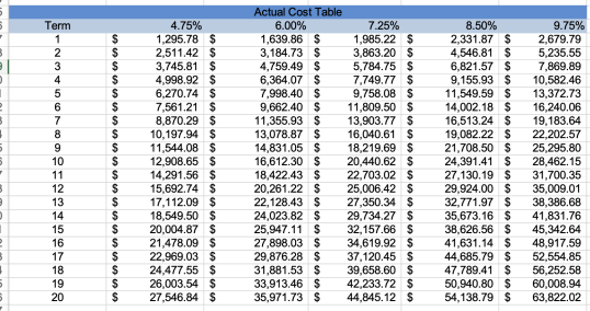
Figure 3: An example of the payment summary sheet for Problem 2 should look like
Problem 4 AI Fluency (10 points)
In addition to learning to use an AI chatbot to create and use functions inside spreadsheets, you will learn to use AI chatbots to enter other fields, such as your major field of study. https://www.anthropic. com/learn provides valuable information on utilizing Claude within and outside the field of computer science. Please complete the course "AI Fluency for students". Pass the AI Fluency course for students by getting your certificate. We will use the terminology of the AI Fluency course in our labs when we reflect on how we use AI.
To demonstrate that you have studied AI fluency, put a picture of your certificate into a cell of your starter file. Create a worksheet called "AI Fluency" and put the picture in cell C3. Use Insert > Illustrations > Pictures > Place in Cell/...
Grading Chats
We grade the chats you turn in (as requested in the assignment). Here is a list of issues we look out for in your chats. The terminology we use: A chat consists of a sequence of pairs of prompts (by the student) and responses (by Claude). We write short chats. The shorter, the better. We don’t want long sequences of pairs. For example, suppose the goal of the chat is to produce a LAMBDA (or any other Excel formula). In that case, we attempt to write an English program in the first chat that contains the complete instructions for generating the LAMBDA.
• A prompt may be ambiguous. What is intended needs to be clarified.
• A prompt may need to be completed. Not all requirements are mentioned.
• The prompt contains only some context information for solving the problem adequately. The context must be complete.
• A prompt should make reasonable requests to Claude. A request NOT to make mistakes is not appropriate. But a request to give hints to solve the problem incrementally is reasonable.
• Chats should cover only one topic. So, there should be a chat for Fibonacci numbers and a separate chat for column statistics. There are generic prompts that apply to many different topics.
• References to earlier text must be unique.
• When Claude returns hints on how to structure an Excel formula, it must be run in Excel 365 to check it. Hint errors must be reported to Claude when you ask for a correction.
• When Claude returns instructions on how to click widgets, you must execute the instructions to check their correctness. Errors must be reported to Claude.
• Instruct Claude to give hints to solve problems incrementally and check each increment.
2025-10-15
Using More Advanced Functions