Hello, dear friend, you can consult us at any time if you have any questions, add WeChat: daixieit

ECON 4400

Problem Set 2

Instructions:

Students will type responses and results to the questions below in a separate document. Make sure the document includes your name, course number, meeting days, and the problem set number. You must create and submit a Stata “do file” for this assignment. All questions and parts must be clearly indicated, along with your name, the problem set number, course, and meeting days, on the “do file”. Data files can be downloaded from the “Data Files” module on the Carmen Modules page.

1 Problem Set Submission

To submit your Problem Set 2:

1. do-file: In Stata, click print and save as or print to PDF

2.  Save the write-up as DOCX or PDF and label as “PS2 first name last name ”.

3.  Upload your Problem Set 2 PDF or DOCX file and Stata  “do-file” on our Carmen course site

2 Write-up

All write-ups need to follow the the below structure.

Write your name (first and last), course number, meeting days, and the problem set number in the title. You must show all your work, demonstrating your knowledge of the subject matter. Additionally, you need to indicate the question number and part along with your response. It is helpful when writing up responses to include the question text, ensuring that you directly address the question. In cases where the question text is long, you need to only include the relevant information. See below for examples.

Questions X

(a) Derive the t-statistic for following hypothesis test to see if xj significantly influences y:

The estimated coefficient using OLS is 20 and the standard error of , se(), is 10. The degrees of freedom are df = N - k - 1.

Answer:

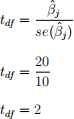
The test-statistic for the jth coefficient is tdf = 2. We reject or do not reject the null hypothesis using either the p-value or critical value methods. Based on our conclusion, xj is a significant or an insignificant factor that influences y.

Make sure to show all your work where applicable. You do not need to show every step but enough that demonstrates knowledge of how to arrive at a solution—round all calculations to four decimal places.

You need to report your regression estimates (at this stage of the course) as follows:

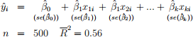
where is the estimated coefficient for xj, for all j = 0, 1, 2,..., k. Report standard errors in parentheses (se(βj)) below the coefficient estimates of .

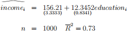
Example:

3 Problem Set 2 Questions

1.  (50 points)  In 2003, Ray Fair analyzed the relationship between stock prices and risk aversion by looking at the 1996-2000 performance of the 65 companies that had been a part of Standard and Poor’s famous index (the S& P 500) since its inception in 1957.

Fair focused on the P/E ratio (the ratio of a company’s stock price to its earnings per share) and its relationship to the beta coefficient (a measure of a company’s riskiness–a high beta implies high risk).  Hypothesizing that the stock price would be a positive function of earnings growth and dividend growth, he estimated the following equations:

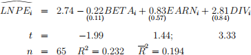
where      LNPEi       = the log of the median P/E ratio of the ith company from 1996 to 2000

BETAi       = the mean beta coefficient of the ith company from 1958 to 1994

EARNi      = the median percentage earnings growth rate for the ith company from 1996 to 2000

DIVi         = the median percentage dividend growth rate for the ith company from 1996 to 2000

(a)  (15 points)  Use the Stock7.dta and replicate the above results in Stata.  Create and test appropriate hypotheses about the slope coefficients of this equation at the conventional significance levels (Hint: one-sided tests).

(b)  (15 points)  One of these variables is lagged and yet this is a cross-sectional equation.

Explain which variable is lagged and why you think Fair lagged it.

(c)  (20 points)  Is one of Fair’s variables potentially irrelevant?  Which one?  Use Stata to estimate Fair’s equation without your potentially irrelevant variable, and then apply the below specification criteria to determine whether the variable is indeed irrelevant.

Specification criteria for deciding whether a given variable belongs in the model.

1.  Theory:  Is the variable’s place in the model unambiguous and theoretically sound?

2.  t-Test:  Is the variable’s estimated coefficient significant in the expected direc- tion?

3. :  Does the overall fit of the equation (adjusted for degrees of freedom) im- prove when the variable is added to the model?

4.  Bias:  Do other variables’ coefficients change significantly when the variable is added to the equation?

2.  (50 points)  Use the birthweight smoking data set introduced in Empirical Exercise E5.3 in the textbook to answer the following questions.  The file contains 3,000 observa- tions on the variables described below

birthweight= birth weight of infant (in grams)

smoker       =  indicator equal to one if the mother smoked during pregnancy and zero, otherwise.

age              = age of the mother

educ           =  mother’s years of educational attainment (more than 16 years coded as 17)

unmarried  = indicator =1 if mother is unmarried

alcohol       =  indicator=1 if mother drank alcohol during pregnancy

drinks        = number of drinks per week

tripre1        = indicator=1 if 1st prenatal care visit in 1st trimester

tripre2        = indicator=1 if 1st prenatal care visit in 2nd trimester

tripre3        = indicator=1 if 1st prenatal care visit in 3rd trimester

tripre0        = indicator=1 if no prenatal visits

nprevist     = total number of prenatal visits

(a)  (5 points)  In Stata, regress  birthweight on smoker and report your results.  What is the estimated effect of smoking on birth weight?

(b)  (25 points)  In Stata, regress birthweight on smoker, alcohol, and nprevisit and re- port your results.

i.  (5 points)  Using the two conditions in Key Concept 6.1 in the textbook, explain why the exclusion of alochol and nprevist could lead to omitted variable bias in the regression estimated in part (a).

ii.  (5 points)  Is the estimated effect of smoking on birth weight substantially dif- ferent from the regression that excludes alochol and nprevist?  Does the regres- sion in (a) seem to suffer from omitted variable bias?

iii.  (5 points)  Jane smoked during her pregnancy, did not drink alcohol, and had eight (8) prenatal care visits.  In Stata, use the regression to predict the birth weight of Jane’s child and report it in your write-up.

iv.  (5 points)  Report and .  Discuss why they are so similar.

v.  (5 points)  How should you interpret the coefficient on nprevist?  Does the co- efficient measure a causal effect of prenatal care visits on birth weight?  If not, what does it measure? Explain.

(c)  (5 points)  Estimate the coefficient on smoking for the multiple regression model in part (b), using the three-step process in the textbook’s Appendix 6.3 (the Frisch- Waugh theorem).   Verify  that  the  three-step process yields the same estimated coefficient for smoking as that obtained in part (b).  (Hint: You will need to use the predict  resids,  residuals command following the reg command to calculate the residuals.  Note, you will want to change the name ”resids” to something else that allows you to predict and add multiple residuals to your data file.)

(d)  (15 points)  An alternative way to control for prenatal care visits is to use the binary variables tripre0 through tripre3.  Regress  birthweight on smoker,  alcohol, tripre0, tripre2, and tripre3 and report your results.

i.  (3 points)  Why is tripre1  excluded from the regression?  What would happen if you included it in the regression?

ii.  (4 points)  The estimated coefficient on tripre0 is large and negative.   What does this coefficient measure? Interpret its value.

iii.  (4 points)  Interpret the value of the estimated coefficients on tripre2 and tripre3.

iv.  (4 points)  Does the regression in part (d) explain a large fraction of the variance in birth weight than the regression in part (b)? Explain.