Workshop 1: A/D and D/A Conversions
Hello, dear friend, you can consult us at any time if you have any questions, add WeChat: daixieit
Workshop 1: A/D and D/A Conversions (15%)
In this project, students are required to design a program to perform analog to digital (A/D) conversion and digital to analog (D/A) conversion on Matlab or Pathon. Specifically, given the input signal x(t)=A1cos(2πf1t)+A2sin(2πf2t) (the way to generate the parameters A1, f1, A2, and f2 will be introduced later), 0≤t≤1, you first need to act as a transmitter to perform the A/D conversion via sampling and quantization. Assume that these quantization bits can be sent to the receiver without any error. Then, you act as a receiver and perform the D/A conversion via de-quantization and de-sampling based on your received quantization bits. You will see what is your estimated signal y(t), 0≤t≤1, and what is the error to the original signal, i.e., y(t)-x(t), 0≤t≤1.
Note that in Matlab and Pathon, there are functions to perform A/D and D/A conversions directly. You are not allowed to call these functions. Please design your code based on the following instructions.
Step 1: Initializing the parameters of input signals. Please generate the parameters A1, f1, A2, and f2 in the input signal x(t)=A1cos(2πf1t)+A2sin(2πf2t), 0≤t≤1, using the first 8 digits of your Student ID. Specifically, A1 is the sum of the first four digits of your ID and A2 is the sum of the last four digits of your ID. Then, convert the last four digits of your ID, which is a decimal number, into a 16-bit binary number (you may do the conversion using the Matlab function “dec2bin” or some online conversion website). For the corresponding 16-bit binary number, f1 is set to be the number of ones and f2 is set to be the number of zeros. For example, if your ID is 21003456, then A1=2+1+0+0=3 and A2=3+4+5+6=18. Moreover, the 16-bit binary expression of the last 4 digits of ID, i.e., 3456, is 00001101 10000000. Thus, f1=4 Hz and f2=12 Hz. Therefore, based on this ID, the input signal is x(t)=3cos(2π*4*t)+18sin(2π*12*t), 0≤t≤1. Please generate the input signal based on your own ID and plot this input signal over the time interval 0≤t≤1 in Figure 1. Show Figure 1 in your report.
Step 2: Sampling. Set fN=2max(f1,f2) Hz. Please sample your input signal x(t) over the time interval 0≤t≤1 at two sampling frequencies: 2fN Hz and fN/2 Hz. Here, you can assume that the ideal sampling technique is employed. For each of the above two sampling rates, please plot all the samples obtained in the time interval 0≤t≤1 in Figure 2. Show Figure 2 in your reports.
Step 3: Quantization. Under each of the above two sampling rates, you need to perform uniform quantization using 4 quantization bits for each sample. For example, when the sampling rate is 2fN Hz, you get 2fN samples from the input signal in the time interval 0≤t≤1. Please use 4 quantization bits to represent each of these samples. Note that the maximum and minimum values of x(t) areA1+A2 and –A1-A2, respectively. As a result, if you have 4 quantization bits, you can divide the regime [–A1-A2, A1+A2] into 24 sub-regimes. Suppose that natural binary coding is used for assigning quantization bits. Please refer to the lecture slides to see how to assign the quantization bits to each sub-regime. Similarly, when the sampling rate is fN/2 Hz, you get fN/2 samples from the input signal in the time interval 0≤t≤1, and you use 4 bits to quantize each sample.
Now, you have two cases: 1. sampling rate is 2fN Hz, number of quantization bits is 4; 2. sampling rate is fN/2 Hz, number of quantization bits is 4. Please show your quantization codebook (how to assign 4 bits each sub-regime) in Figure 3 of your report. Then, for each of the above two cases, please show the quantization bits for all the samples in your report (suppose that natural binary coding is used).
Step 4: De-quantization. Suppose that the receiver can receive all the quantization bits without error. Then, you need to perform de-quantization based on the received quantization bits using the same quantization codebook as the transmitter. For both sampling rates 2fN Hz and fN/2 Hz, please show in the report the recovered samples over the time interval 0≤t≤1 in Figure 4.
Step 5: De-sampling. Based on the recovered samples, the receiver can perform de- sampling to get the estimation of x(t) over the time interval 0≤t≤1. Please refer to the lecture slides for how to do the de-sampling. Please show your estimated signals over the time interval 0≤t≤1 at the two sampling rates in Figure 5.
Important Notes: Due to time limitation, this workshop can be finished in two parts. The first part is about Steps 1 – 4, and the second part is about Step 5. The students have to finish the first part in the lab during the 3-hour period in Workshop 1. Then, the students can copy their codes and finish the second part after Workshop 1. The second part has to be submitted to Blackboard before 11:59pm, February 24, 2025.
Submission Checklist 1 (Step 1 – Step 4; show to the TAs at the lab):
1. Your Matlab or Pathon code
2. Your name and student ID
3. Figures 1 to 4 as required in Steps 1 - 4. Note that in Figures 2 and 4, each figure should show two sampling rates.
4. The quantization bits for all the samples in Step 3, under two sampling rates.
Submission Checklist 2 (Step 5; submit on Blackboard)
1. Deadline: 11:59pm, September 23, 2025
2. Visit the website of our course at blackboard. On the left tool bar, click on “Assessment”. You will see an item “Please submit Workshop 1 here” . Attach the following documents there.
2.1 Your Matlab or Pathon code
2.2 Your name and student ID
2.3 Fig. 1 required in Step 1 and Fig. 5 required in Step 5. In Step 5, you should show the recovered signal under two sampling rates.
Example: In this example, we set A1=3, A2=4, f1=2, f2=5 in the input signal, i.e., x(t)=3cos(2π*2*t)+4sin(2π*5*t), 0≤t≤1. The sampling rate is 2fN=20 Hz. Each sample is quantized by 4 bits. Figures 1, 2, 4, 5 (quantization codebook and quantization bits for all the samples are omitted here) are shown as follows:
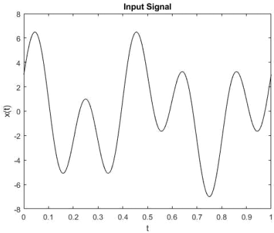
Figure 1
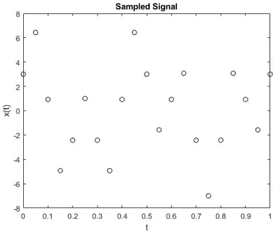
Figure 2
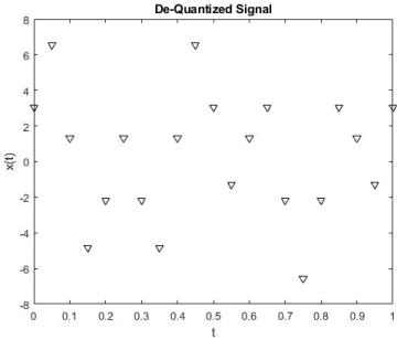
Figure 4
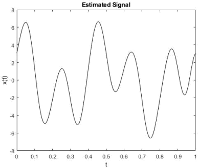
Figure 5
2025-09-25