Hello, dear friend, you can consult us at any time if you have any questions, add WeChat: daixieit

PHY146

EXPERIMENT

Free Fall and Projectile Motion

Introduction:

1. Free fall

We will start as usual, with Newton’s 2^nd Law:

 (1)

For free fall, the only force on the object is gravitational, and acceleration is the 2^nd derivative of position, so

 (2)

 (3)

Integrating twice yields

 (4)

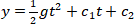 (5)

Note that by plugging in t = 0, we can deduce that c1 = v0 and c2 = y0. If v0 = 0 then it follows that

 (6)

Whenever the air resistance on a falling object is negligible, the motion is referred to as free fall. Near the earth’s surface, the acceleration due to gravity “g” is nearly constant over the range of motion and approximately equals 9.80 m/s² downward. This value decreases with increasing altitude and slightly varies with latitude. A freely falling object moves freely under the effect of gravity regardless of its initial condition. For a freely falling body, the same kinematic equations, mentioned above, hold true with the substitution a = - g.

2. Projectile Motion

The horizontal range, Dx, for a projectile can also be found starting from Newton’s 2^nd Law:

 (7)

 (8)

 (9)

 (10)

Noting that dt/dx is a constant, we will say c1 = vx, and plugging in t = 0 as before yields c2 = x0, therefore

 (11)

where v_x is the horizontal velocity and t is the time of flight.

To find the time of flight, t, we will use the same equation we derived for free fall:

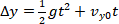 (12)

where Dy is the height, g is the acceleration due to gravity and v_y0 is the vertical component of the initial velocity.

When a projectile is fired horizontally (from some height), the time of flight can be found from rearranging Equation 12. Since the initial vertical velocity is zero, the last term drops out of the equation, yielding:

 (12a)

When a projectile is fired at an angle and it lands at the same elevation from which it was launched, Δy = 0. Rearranging equation 12 yields:

 (12b)

3. Uncertainty

One of the most important parts of this experiment is the error analysis. For any measurement, there are two types of uncertainty to consider. The first is the reading error, which quantifies how precisely your measuring device can tell you information. The reading error is defined as half of the smallest increment of the measuring device. The second type of uncertainty comes from fluctuations in the data itself. This is referred to as the standard error or the standard deviation of the mean sx, can only be measured with multiple readings, and is given by

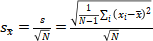 (13)

where s is the sample standard deviation, xi is the i^th measurement, x is the sample mean, and N is the number of measurements taken. Generally speaking, either the reading error or the standard error will dominate, and the other one can be ignored. If you’re not sure which to use, take a few measurements without changing any experimental conditions. Figure out which one is larger, and use it. Note that it is possible to reduce the standard error indefinitely by taking more measurements, but for the purposes of this course, we can limit ourselves to say 5 trials. Up to this point, we are either considering only the reading error on a single measurement, or the standard error on the average of several measurements, and we will consider the uncertainty of any given measurement to be the larger of the two types of error. When we include this data on a graph, we will show the uncertainty as an error bar along the appropriate axis (frequently we will have both x-axis and y-axis error bars).

Often we will want to find the uncertainty on the slope of a line of best fit. This is accomplished by doing linear regression. The slope’s uncertainty sm is given by

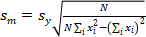 (14)

where sy is the standard deviation of the y-values.

Also note that sometimes we will be calculating new quantities to plot, i.e. we won’t always be plotting our values directly. In this case, we will need to propagate the uncertainties on our measured values through to find the uncertainties on our plotted values. The general error propagation formula assumes that we have a function

 (15)

and is given by

 (16)

This formula will work for all uncertainty propagation, however, a number of special cases are shown in the Uncertainty document on Quercus. Also note that you will need to use error propagation to calculate the uncertainty on your final answer from the uncertainty on your slope (unless your slope happens to be the exact quantity you’re looking for).

Important note: all of this uncertainty theory applies to all the experiments in this course.

Procedure:

Exercise 1: Free Fall

The equation of motion for a body free-falling from rest can be expressed as in equation 6, where y is the distance the object has traveled from its starting point, g is the acceleration due to gravity, and t is the time elapsed since the motion began. In this experiment, you will find an estimate for g by carefully timing the fall of a steel ball from various heights.

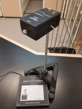
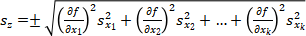
Fig. (1) Equipment Setup

The following steps describe how to measure the free fall time of an object with the experimental setup:

1. Clamp the ball release mechanism to a lab stand, or any other device that will hold it at the desired height over the table, as shown in figure 1.

2. Ensure that the two leads from the trigger are plugged into the Control Box and port 1 of the data acquisition interface, and that the time-of-flight accessory is plugged into port 2.

3. Position the time-of-flight accessory directly under the ball.

4. Set the Control Box to Active. Ensure that the equipment is set up as per figure 2, below.

5. Open the Capstone file called Free Fall (from Blackboard).

6. Place the steel ball on the release mechanism at the bottom of the drop box. Wait until the LED on the drop box stops blinking. Press the Record button in Capstone.

7. Press the trigger to drop the ball. If it doesn’t drop, you may need to unplug the Control Box and plug it in again.

8. Read the time on Capstone’s table display. This is the time it took for the ball to fall from the bottom of the drop box to the time-of-flight accessory.

9. To time another drop, return the ball to the drop box and press the trigger again. It is best if you don’t press stop between trials for a specific height; that way all your numbers for one height will be in one run and display in one table.

Fig. (2) Equipment Setup, continued

1. Set up the free fall timer as described above.

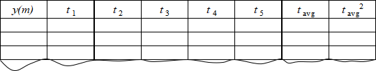
2. Set y, the height from the bottom of the ball to the time-of-flight accessory, to the highest position you can achieve on the table (using the supplied stand; if you use larger stands there is a risk of damage to the time-of-flight accessory). Measure the distance as accurately as possible and record the distance in Table 1. Here we are measuring a distance, so we will assume that the standard error is small, and quote the uncertainty as the reading error. Record the time it takes for the ball to drop as t₁ in Table 1. Repeat the measurement at least four times and record these values as t₂-t₅. Calculate the average of your five measured times and record this value as t_avg. In addition, calculate the standard error of these measurements (here we will assume that the reading error of the time measurements is small and quote the uncertainty as the standard error). Once you have t_avg and its uncertainty, use the error propagation formula (equation 16) to calculate the uncertainty on t2avg. Note that the Uncertainty document on Quercus contains error propagation formulas for several specific situations, all of which are derived from equation 16 but may make your life easier. In this case, you would use the exponent formula.

3. Set y to at least 10 different heights, repeating step 2 for each value of y. Of course, the more heights you use, the better the results you will get.

Table 1 Data and Calculations

Make sure to perform the following steps for your lab report:

Plot a graph of y versus t2avg with y as the dependent value (y-axis). Make sure to include the reading error of your position measurement as the error bar along the y-axis, and the error on t2avg as the error bar along the x-axis. Within the limits of your experimental accuracy, do your data points define a straight line for each ball? Was the acceleration constant?

If your graph was linear, measure the slope. You will also need to find the uncertainty on the slope. To do this, use linear regression. Using your measured slope and the equation shown in the introduction to this experiment, determine the acceleration caused by gravity. Be sure to include the units and an estimate of uncertainty, and compare your measured value to the accepted value of g.

Here are some things to think about when writing:

1. Is the acceleration caused by gravity constant?

2. Discuss the conditions under which you believe your results to be true.

3. Include a discussion of the errors in your measurements and how they affect your conclusions.

Exercise 2: Projectile Motion

Setup

Most of the setup should be prepared for you, however these instructions are here for reference.

1. Choose one corner of a table to place the projectile launcher.

2. Clamp the launcher to the corner of the table using the Universal Table Clamp (see photo below).

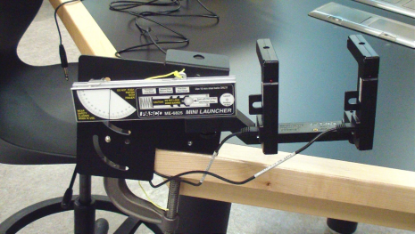
Fig. (3) Equipment Setup, continued

3. Slide the Photogate Bracket into the groove on the bottom of the launcher and tighten the thumbscrew.

4. Connect two photogates to the bracket.

5. Plug the photogate closest to the launcher into port 3 of the data acquisition interface. Plug the other photogate into port 4.

6. Adjust the height of the launcher and/or the time-of-flight accessory so that the ball launches from and lands at the same elevation. Place a barrier at the other end of the table to prevent the steel ball from rolling away.

7. Adjust the angle of the launcher to 25^o or less to start with. You will need to cover as wide a range as possible, up to, say, 85 ^o. Note: With the photogate bracket and photogates attached to the launcher and the launcher in the lower track and pointing directly into the table, the lowest angle is approximately 23^o. You may be able to achieve lower angles by clamping the launcher to one side of a table.

8. Note that you should adjust the launcher and/or place the time-of-flight accessory on top of other items such that the first photogate and the time-of-flight accessory are at the same height.

Launching at an Angle

1. Record the spacing between the two photogates.

2. Using the push rod, push the ball into the Launcher until it clicks once. Using the string, pull back on the trigger. Note the location on the table where the ball lands.

3. Place the time-of-flight accessory at this location. Tape a sheet of blank paper on top of the time-of-flight accessory. Place carbon paper over the blank paper.

4. Open the Capstone file called Projectile Motion (from Blackboard), and press Record (note: you MUST load the ball before pressing Record because otherwise blocking the photogate will start the timer and your readings will be useless).

5. Launch the ball. Press Stop in Capstone.

6. Use the tape measure to find the horizontal range (the distance from the launch position to the black mark that the carbon paper makes on the white paper.

7. Record the the horizontal range, and the time of flight, either in your notes or by saving the file (I recommend both for redundancy).

8. Repeat steps 1-7 for at least 7 different angles over as wide a range as possible.

9. Set the launcher to zero degrees (horizontal) and record the time between photogates. Do this five times so that you can calculate the standard error; again we will assume that the reading error is small for the time. Why do we only want this value for zero degrees?

Make sure to perform the following steps for your lab report:

1. Measure the distance between the photogates and record its uncertainty. Using that value and the time it takes for the ball to travel between the photogates, calculate the initial velocities of the ball for each angle, and their uncertainties using equation 16 or the specific examples in the Uncertainty document. In this case, you would use the division formula.

2. Using the initial velocity and the angle; calculate the horizontal range in meters. Hint: Calculate the components of the initial velocities. As always, make sure to calculate the uncertainty using equation 16.

3. Plot both the Measured Horizontal Range vs. Angle and the Calculated Horizontal Range vs. Angle on the same graph. As always when plotting experimental data, make sure to include error bars. The error bars along each axis should be the uncertainty in the quantity plotted on that axis.

4. Also, plot the Time of Flight vs. the y-component of the initial velocity. What is the slope of this graph? As before, use linear regression to find the uncertainty on the slope.

5. Refer to your Angle vs. Range graph. What angle corresponds to the maximum range? Explain why this particular angle produces the maximum range. Are your theoretical and experimental values consistent within experimental uncertainty?

6. From your Time of Flight graph, calculate g and its uncertainty.

REFERENCES :

[1] Stillman Drake, “A History of Free Fall: Aristotle to Galileo” Wall and Thomson, 1989.

[2] Giancoli D.C.“Physics for Scientists and Engineers” 2^nd Ed., Prentice Hall Inc., 2003.

[3] Serway R.A. , “Physics for Scientists and Engineers / with  Modern  Physics” Saunders

College  Publishing, 2004.

[4] Halliday D.and Resnick R.,“Fundamentals of Physics” 7^th Ed.,Wiley and sons, N.Y.,2005.