GGR112 Assignment 1 Lab 1: Topographic and Thematic Map Primer
Hello, dear friend, you can consult us at any time if you have any questions, add WeChat: daixieit
GGR112 | Assignment 1
Lab 1: Topographic and Thematic Map Primer
Grading:
Answers to the questions in this assignment are to be submitted via Quercus. While working in your practical session, you can jot your answers down in your notebook or your computer.
Due Date:
The assignment due date depends on the day of your practical, as outlined in the syllabus.
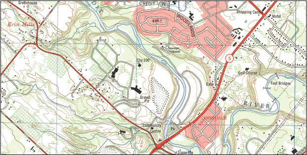
Figure 1: Vintage topographic map sheet of the area around campus depicting our orchards and local gravel pit. Elevations are in feet, Erindale Park has a sewage treatment plant in it and Erin Mills Parkway is a dirt road.
Introduction:
Topographic maps depict the landscape at a local scale and use a projection that allows for distance measurement and navigation. They are the all-purpose map, providing a comprehensive overview of the landscape and its features. Topographic maps are free, and in Canada, as in most nations, topographic maps are published by a branch of government (Federal in Canada) and have traditionally been distributed as printed sheets. Many modern digital products borrow their feature databases, conventions, symbology and even aesthetics from topographic maps.
Objective:
Become familiar with topographic maps, be able to visualize the landscape and understand the basics of scale, elevation, features and navigating using a map. Compare topographic and thematic mapping.
Background:
Canadian topographic maps produced by Natural Resources Canada have the goal of accurately depicting “…ground relief (landforms and terrain), drainage (lakes and rivers), forest cover, administrative areas, populated areas, transportation routes and facilities (including roads and railways), and other man-made features.” 1 They are published at 1:50 000 and 1:250 000 scale. The 1:50 000 scale maps are most common and are used for recreational, planning, natural resource management, emergency response and land-use planning purposes. At 1:50 000, 1 cm on the map is equivalent to 50 000 cm or 500 metres or 0.5 km in the real world and one 29” x 36” map sheet depicts about 1000 km2 . Contemporary digital products used in GIS systems are derived from topographic maps as well; building on nearly 100 years of surveying and observations in the local area.
Materials:
The National Topographic System of Canada subdivides the nation into a series of alphabetically and numerically designated ‘map sheets’ called NTS map sheets. In this practical you will be the 30 M/12 1:50 000 ‘Brampton’ sheet.
• 30 M/12 ‘Brampton’ Topographic Map Sheet (Edition 7)
o available in DV2062 and following the practicals in the Library Tech Centre Room (HMALC room 360)
• Legend for above map
• Graph paper
• Blank paper
• Metric Ruler
• String for measuring distances along non-straight lines
• Topographic Maps: The Basics – Natural Resources Canada Publication © 2014 Her Majesty the Queen in Right of Canada, as represented by the Minister of Natural Resources Canada
• Video guide for creating topographic profiles (http://uoft.me/GGR112Lab1)
Section 1 | Orientation
Background
Begin with the margins. The topographic sheet features the title, scale and other metadata alongside the map. The title is at bottom right along with publishing information and the year of production. Directly above this is a diagram showing adjacent map sheets by their index number.
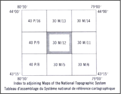
Figure 2: You are using sheet 30 M/12, directly to east is 30 M/11 to the north is 30 M/13 etc.
Above the adjacent map sheet reference are instructions on how to use the Universal Transverse Mercator (UTM) coordinate reference system.
Answer the following questions (1 point each):
1. What is the title of this map sheet?
2. What is the NTS map sheet reference?
3. Which edition is the map sheet?
4. Which map sheet is directly to the south of 30 M/12?
5. When was it published?
Section 2 | Coordinates, Grids and Distance
North is aligned to the top of every topographic map published in Canada. Figure 3 (left) shows the north adjustment required to use a compass with the map as magnetic north as indicated by a compass differs from true north and moves slightly each year. You will also see the compass reference orienting you to north on the map. There are three types of North on a Canadian topographic sheet. Figure 3 (right) depicts a compass rose with intermediate bearings. With the map sheet aligned with north at the top (normal orientation) east will always be to the right, west to the left and south at the bottom of the sheet.
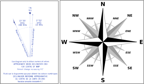
Figure 3: (Left image) Three varieties of north found on a topographic map. True north is always oriented to the top of the map sheet. Grid north is the north orientation of the UTM coordinate grid for the particular map sheet. Magnetic north is a slowly changing bearing representing the location of the magnetic north pole toward which a compass needle or your phone compass will point. To navigate using a topographic map and compass you must account for the difference between magnetic and grid north. (Right Image) a compass rose to help you refer to relative direction for this assignment.
Moving further up the edge of the map sheet you will find the geographic coordinates written along the periphery of map image. Figure 4 indicates that the top right corner of the map is at 79° 30’ West and 43° 45’ North. This is read as “79 degrees 30 minutes west and 43 degrees 45 minutes north”. The first coordinate is the longitude and represents our distance west from the 0° line of longitude which passes through Greenwich, UK and is also the origin point of our time zone system. The second coordinate is latitude, or the distance in degrees north of the equator (denoted as 0° latitude). Each degree (°) can be subdivided into 60 minutes (‘) and those further subdivided into 60 seconds (“). While very useful for locating features on a global scale, the lines of longitude converge near the poles and thus do not lend themselves to distance measurement – the on-the-ground distance of a single degree or minute of longitude diminishes as a you travel closer to the poles.
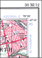
Figure 4: In the corners of the map you will find both the latitude and longitude (in black serif font) as well as UTM coordinate system grid reference (in blue sans-serif font). The coordinates at the four corners of the map are referred to as the extent of the map – the term carries over to GIS uses and indicates the coverage area of the map sheet or data set.
In order to make topographic maps usable for navigation and direct on-map distance calculation, a second coordinate system is used – referred to as the Universal Transverse Mercator Grid Reference System, or simply the UTM grid. You can see this along the edge of the map as blue numbers and letters. The UTM grid subdivides the entire world into a series of 60 zones, each representing 6° of longitude and numbered from 1 to 60, beginning at the south pole, zones are labelled B to Z traveling north. An excellent overview of this is included in the appendix to this assignment. Canada is large enough to be present in zones 7 through 22, a total of 16. Our campus, and this map sheet are located in zone 17T.
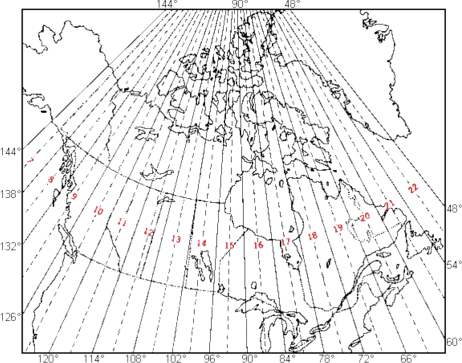
Figure 5: Canadian UTM Zones; our campus and Toronto are located in zone 17 in the northern hemisphere. This is often referred to as UTM zone 17T, with the letter T corresponding to the latitudinal band.
The UTM grid uses meters as its unit of measurement rather than the degrees, minutes and seconds used in the geographic coordinate system. Within any given UTM grid (e.g., 17T), position can be referenced using grid coordinate pairs. Coordinate pairs include a 'northing' and an 'easting'. In the northern hemisphere, the northing coordinate represents the metric distance in meters from the equator (increasing poleward), and the easting coordinate represents distance from the western edge of the UTM zone.
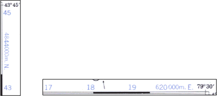
Figure 6: (Left) The northings and (right) the eastings of the UTM grid coordinate system on the 030M12 map sheet
The UTM grid divides the map into equally sized squares making locating features easy. Along the right edge of the map the UTM gridline marked 4844000m N implies that we are or 4 844 000 metres (4844 km) north of the equator. The full number is written only a few times along the edge of the map, it is used in a shortened otherwise (the ‘45’ and ‘43’ written above and below this value represent 4 845 000 N and 4 843 000 N respectively). The east-west axis is the same, but all values are a distance from the western edge boundary of the UTM zone. Figure 6 (right) shows that near the top right or north east corner of the map, the gridline is located at 620 000 E. Just like the northings, the eastings are in shortened form – the line just to the west or 620 000 E is 619 000 E. As you have probably figured out, each square is 1000 m or 1 km per side, and each grid line is separated by 1000 m or 1 km.
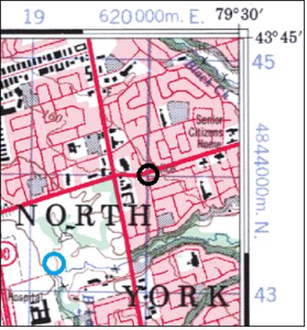
Figure 7: Example of UTM coordinate location
To locate a feature at the intersection of two lines is simple. According to UTM conventions, the location of the black circle in Figure 7 is noted as follows:

In-line with text you would write is like so: 17T 620000E 4844000N. This coordinate system can be used to locate a feature anywhere in the world.
To locate a feature not at the precise intersection of two UTM grid lines (like the blue circle in Figure 7), you subdivide each square into 10ths. You can do this using a ruler (as in Figure 8), or by estimating visually. If we estimated the location of the blue circle we would note it as follows:
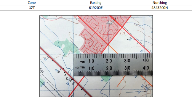
Figure 8: 1:50000 scale NTS sheets grids are exactly 20 mm or 2 cm per square. This means that 2 cm = 1 km
Using a ruler, each 1 mm is equivalent to 50 metres. In the above example, the road intersects the ruler approximately 16mm from its 0 mark which I have lined up with the 592000E UTM grid line – 16mm is equivalent to 800 meters. The easting for this road would be noted as 592800E.
Answer the following questions (1 point each):
6. On the Brampton 1:50000 map sheet, 225 mm is equivalent to how many kilometers?
7. What is the name of the community located at 593300E 4824500N?
Locate Lester B. Pearson International Airport.
8. One of the runways at the airport is exactly parallel to the UTM grid; which northing grid line is it parallel and adjacent to?
9. How long is this runway in kilometres?
10. What are the names of the two creeks which pass through Pearson International Airport?
11. Which is the wider of the two streams?
12. What is the feature at 584900E, 4841600N?
13. From this point, in what direction is the Mississauga community of Meadowvale West?
14. What is the approximate elevation at 620500E 4826500N rounded to the nearest metre?
Locate the UTM campus (known as Erindale College when the map was produced).
15. Provide the easting for the chimney on site.
16. Provide the northing for the chimney on site.
17. Using a string to conform to the curves of the Credit River, determine the distance in kilometers by canoe from the campus to Lake Ontario.
18. Name the creek which flows into the Credit River just downstream from campus.
Locate the water body at 583500E 4818000N.
19. What is the name of the conservation area that this water body is located in?
20. What is the feature located at the southeast edge of this water body?
21. What is the approximate elevation of this water body?
22. Another smaller water body is located 1.2km east of this one. Is it higher, lower or equal in elevation?
23. What is the name of the creek flowing out of Kelso Lake?
24. There is a ski hill at this conservation area. What is the elevation drop from the top of the hill to the railroad tracks at the bottom? Pro tip – refer to the next section and Topographic Maps: The Basics if you are unclear on how to determine elevation.
Section 3 | Elevation and Contour Lines
A key feature of topographic maps is elevation information. In contrast, planimetric maps such as road maps or transit maps do not include this important landscape characteristic. Elevation is reported in several formats on the topographic map sheet. Spot elevations mark peaks, low points, significant topographical features, towers and vertical benchmarks used for surveying or construction purposes. You can find these all on the legend. However, these only provide elevation at a single point, which is of limited utility.
To aid the user in visualizing the landscape, topographic map sheets depict elevation data using contour lines (depicted in brown). They depict elevation information for the entire map sheet and allow the user to determine which direction the land slopes (the aspect of the slope), the steepness of slope (amount of elevation change for a given horizontal distance) and therefore can be used to answer practical hydrological questions such as what is the direction of drainage. Here are some key points to remember about contour lines:
• a contour line connects points of equal elevation relative to a given reference plane (usually mean sea level or MSL)
• we refer to elevations on the map as metres above sea level, eg. 350 m ASL
• they never branch or split
• they always form a continuous shape (they do not end but may extend beyond the margins of a given map sheet)
• thicker contour lines represent an index contour – typically every 50 metres (100 m, 150 m, 200 m etc.)
• various maps have differing contour intervals, this map uses a 10 metre interval
o this implies that the gap between two contour lines on this map sheet always represents an elevation difference of 10 metres
o therefore… if contour lines are closely spaced, the gradient is steep (10 metre elevation changes are frequent) if contour lines are spaced widely apart the gradient is very mild (10 metre changes are infrequent)
• as a rule, contour lines will encircle elevations which are higher than the value of the line
o depressions (for example a lake located on a hilltop) on elevated parts of the landscape are an exception, and are clearly marked on the map with a contour line that is hashed (refer to the legend for an example)
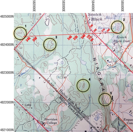
Figure 9: Elevation example
Figure 9 shows examples of several methods that topographic maps use to depict elevation information.
1. This point indicates a local peak, situated within the bold contour for 350 m elevation, this peak sits 5 m higher at 355 m. This ‘precise elevation’ is shown on the map because it is locally prominent – the highest point in the landscape and was likely surveyed as a reference.
2. This elevation value depicts the approximate elevation of the surface of the Scotch Block Reservoir. You will find elevations listed for numerous bodies of water. These numbers will help you determine the value of the contour lines surrounding water bodies. The red transect between the two points illustrates how contour lines are used to depict changes in elevation.
3. Index contours on this map sheet are thicker and represent 50m intervals, there will always be 4 intermediate contour lines between two index lines of different elevation – pay close attention to this, since we can see that in this region of the map the landscape varies between 340 m and 350 m – we can tell that these index contours have the same elevation because they are not separated by 4 intermediate contours.
4. The most helpful and direct presentation of elevation data is the labelled contour line. In this case showing an elevation of 330 m. These are not as a common as one would like them to be. Find these in order to orient yourself in an unfamiliar region of the map. The wide spacing of the contour lines in this area of the map indicates a relatively mild slope in contrast to point 5.
5. A very steep gradient is represented by bunched contour lines. Here, over a horizontal distance of approximately 400-500 m the elevation from 320 m to just over 250 m. Note the index contour for 300 m and 250 m (located just to right of the circle).
Answer the following questions (1 point each):
25. How many intermediate contour lines will you find between two index contour lines?
Locate the creek at 582300E 4837000N.
26. What is the name of the creek?
27. To the west of the coordinate is a small reservoir or pond through which the creek flows. What is its elevation?
28. How many metres elevation does the creek drop from the reservoir to where it joins Silver Creek?
29. At what elevation do the two creeks merge?
30. Silver Creek feeds a small wetland area. Provide the range of elevations for the wetland using the nearest contours.
Section 4: Creating a Topographic Profile
One of the primary goals of topographic maps is to allow the user to visualize the landscape. If you have a transect in mind, for example a hiking trail or a planned road route, you can transfer the top-down view of a topographic map to a profile view of the elevation change in the landscape using graph paper. This procedure can also be used to determine slope. The process is simple. You will need 2 pieces of paper, one blank, and one graph. Here is a helpful video guide: http://uoft.me/GGR112Lab1
Answer the following question (10 points):
31. Using the provided grid paper, create an elevation profile along easting line 589000E and from northing 4831000N to 4837000N. The x-axis should be labelled in kilometers with 0 km representing the start point of your profile (i,e., 589000E, 4831000N). Each grid square on the y-axis should represent 5 m of elevation change. On your profile, indicate the positions of any significant waterways (i.e., waterways named on the map) and urban areas. Label the diagram and all axes appropriately. On your grid paper, write your name and sign the profile. Take a good quality (well-lit, well-aligned) cell phone image of your topographic profile and upload to Quercus.
2025-09-20