Hello, dear friend, you can consult us at any time if you have any questions, add WeChat: daixieit

ECO 4421

Econometrics

Assignment 1

Due: 11:59 PM, September 8th, 2025

Instruction

Guidelines   Show all the steps to arrive at the answer step-by-step. You are encouraged to discuss this assignment with your classmates; however, do not copy solutions. If you work on this assignment with your classmates, please list their names at the top of the first page of your PDF file. Each student must submit their own work through Canvas. If any questions ask you to “repeat,” “observe,” or similar actions (especially in R-related questions) and you are unsure what to write, they are simply instructing you to actually “repeat” or “observe” the task–not to write anything specific. (Although this problem set is graded, its primary purpose is to support your learning and study.) The total score for this assignment is 100 points. You will receive 20 points for submitting your solutions on time.

Submission   Please submit three separate files on Canvas - Problem Set 1:

1. A PDF file containing answers to 1, 2, 3, and 7, prepared using LATEX.

2. The knitted .html file containing answers to 4, 5, and 6. If any part of the code does not execute successfully or fails to render in the HTML output, comment it out rather than leaving it as-is. This approach allows the rest of the script to run without errors, ensuring that partial credit can still be awarded based on the attempt. Maintaining clarity and structure in your submission will improve readability and reproducibility.

3. The .rmd file containing answers to 4, 5, and 6. Ensure that your script is well-commented so that each section clearly corresponds to a specific question. At the beginning of the script, include the library() calls for any packages used. Do not include install.packages().

Late submissions will not be accepted under any circumstances.

Generative AI   If you encounter difficulties while programming in R, you are encouraged to utilize resources such as Google, R’s help() function, or reach out to me for assistance. However, the use of generative AI is strictly prohibited for this assignment. Using generative AI as a beginner programmer is highly discouraged, as it may hinder your learning process. Any unauthorized use of generative AI may be considered cheating and/or plagiarism. Such violations of the UF Student Honor Code will be reported to the UF Dean of Students Office and may result in severe sanctions. Generative AI tools include, but are not limited to, ChatGPT, DALL-E, and Google Bard.

1 Summation Operators (10 points)

We explore the summation operator by verifying whether the following equalities hold:

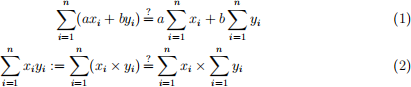
Consider the following data.

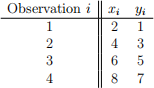
(a) Let a = 3 and b = 2. Compute the left-hand side for (1): 

(b) Let a = 3 and b = 2. Compute the right-hand side for (1):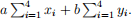 

(c) Let n = 2. For general values of a, b, xi , and yi , expand the left-hand side of (1) without using specific data: 

(d) Let n = 2. For general values of a, b, xi , and yi , expand the right-hand side of (1) without using specific data: 

(e) Is the equality (1) necessarily true? Explain briefly your reasoning.

(f) Compute the left-hand side for (2): 

(g) Compute the first-term of (2): 

(h) Compute the second-term of (2): 

(i) Compute the right-hand side for (2): 

(j) Let n = 2. For general values of xi and yi , expand the left-hand side of (2) without using specific data: 

(k) Let n = 2. For general values of xi and yi , expand the right-hand side of (2) without using specific data: 

(l) Is the equality (2) necessarily true? Explain briefly your reasoning.

2 Population, Sample, and Estimators (10 points)

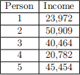
Suppose we are interested in the proportion of poor households in the classroom. The Federal Poverty Line is $32,150 for a family of four. Out of a population of 40 students in a classroom, assume the true proportion of students below this threshold is α = 0.25. Now suppose you randomly select a sample of n = 5 students and observe the following incomes (in dollars):

(a) What is P(X ≤ 32,150)?

(b) Why can we calculate P(X ≤ 32,150) in the population setting but not in the sample setting? What role does the “plug-in principle” play in bridging this gap? Explain briefly in one or two sentences.

(c) If two different groups of 5 students are sampled, will the resulting estimates be the same or different? Why?

(d) Which source of uncertainty do we face in statistics that we do not face in probability? Explain briefly in one sentence.

(e) Is the parameter α a number or a function?

(f) Write the estimator of α using the plug-in principle in summation form.

(g) Compute the estimate of α using the given sample.

(h) Suppose you drew a different sample. Would the estimator change? Would the estimate change? Explain why briefly but clearly in one or two sentences.

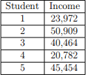
3 Comparing Estimators (10 points)

Suppose we want to estimate the proportion of poor households in the U.S., denoted as α. The Federal Poverty Line is $32,150 for a family of four. You randomly select a sample of n = 5 people and observe the following incomes (in dollars). Let Xi denote the income of person i in the sample.

To estimate α, two estimators are proposed:

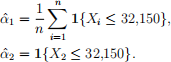
Note that 1{statement} denotes the indicator function, which equals 1 if the statement is true and 0 if it is false.

(a) Interpret what ˆα1 represents and compute its value using the sample.

(b) Interpret what ˆα2 represents and compute its value using the sample.

(c) Suppose the true α = 0.10. With the realized sample above, which estimator gives a value closer to α in terms of absolute difference?

(d) Which estimator would likely be more stable if we repeated sampling many times? Explain briefly in one or two sentences.

(e) If the sample size grows very large, what would you expect from ˆα1 compared to ˆα2?

(f) Which estimator would you prefer and why? (Any reasonable answer will receive full credit. Formal criteria for comparing estimators will be discussed in Module 2.)

4 Population (10 points)

The questions below ask you to select and manipulate variables and use some of R’s functions.

(a) If you are new to R Markdown, log into Canvas and read this page:

https://ufl.instructure.com/courses/534809/pages/r-markdown-guide

(b) Download the population data from Canvas and save it to your R working directory. (Two files contain the same data. Download one of them.) To identify your R working directory, type getwd() in the R console; this will display the current directory. Then, create a variable to store the data. For example, you can use the following code in R:

1   population <- read.csv("data1.csv")

2   load("data1.RData")

After then, clicking on “population” in the Environment shows you the dataset in detail.

(c) You can select each variable in the dataset using the $ sign. For example, to the select the variable education, run the following:

1 population$education

Compute the average number of education using the function mean(). Plot a histogram of education.

(d) You can add a variable using the $ sign and ‘< −’. Add the squared of the level of education as the third variable of the population. What is the average number of the education squared?

1 population$education_squared <- (population$education)^2

(e) You can calculate the sum of all observations in each column using the following:

1 colSums(population)

What is the sum of wages of all observations?

(f) Run the following:

1 summary(population)

Briefly explain what the summary() function does.

5 Discrete Probability Distribution (10 points)

In this question, you will practice R programming, simulation, and explore the Law of Large Numbers. The Law of Large Numbers states that as the sample size increases, the average of the observed results approaches the true value. As you work through this exercise, keep in mind the distinction between “theoretical” (or true) values and the numbers obtained through simulation. The theoretical values are provided in the question (e.g., p = 0.3) or can be calculated analytically (e.g., by hand or using R built-in functions such as dbinom()). However, simulations will rarely yield exact theoretical values; instead, they produce results based on random sampling. Reflect on how the simulated numbers align with the theoretical values and observe how these results change as the sample size increases.

(a) Bernoulli Distribution: Imagine a factory produces light bulbs, where each bulb has a 30% probability (p = 0.3) of being defective and a 70% probability (1 − p = 0.7) of being non-defective. Use the sample() function to simulate a single test of whether a randomly selected light bulb is defective (1 = defective, 0 = non-defective). Repeat this test for a large number of bulbs (e.g., 1000 trials). Compute and observe the empirical proportion of defective bulbs from your simulation. (Since the outcome is either 0 or 1, you can use the mean() function in R to compute the empirical proportion.) How does this compare to the theoretical probability of p = 0.3? (Hint: Look at the Hint file in Canvas for explanations and examples of sample() and mean().)

(b) Law of Large Numbers: Compute the mean number of defective bulbs for increasing sample sizes N = 100, 1000, 10000, and 10000000. Analyze how the proportion of defective bulbs changes as the sample size increases, and compare the results to the theoretical probability of the Bernoulli distribution with p = 0.3.

(c) Binomial Distribution: Imagine a quality control inspector tests a batch of 10 light bulbs at a factory, where each bulb has a 30% probability (p = 0.3) of being defective and a 70% probability (1−p = 0.7) of being non-defective. Use the sample() function to simulate one test of the batch, where you count the number of defective bulbs (successes) in the batch of 10. Repeat this process for a large number of batches (e.g., 1000 trials). Compute and observe the empirical distribution of the number of defective bulbs in each batch. Create a histogram to visualize the results. (Hint: Look at the Hint file in Canvas for explanations and examples of replicate() and sum().)

(d) Create histograms for increasing sample sizes, N = 100, 1000, 10000, and 10000000, while keeping the number of bulbs in each batch fixed at 10. Analyze how the his-tograms compare to the theoretical Binomial distribution with parameters n = 10 and p = 0.3, denoted as B(10, 0.3). (Hint: Refer to the Hint file in Canvas for explanations of the theoretical Binomial distribution.)

6 Continuous Probability Distribution (10 points)

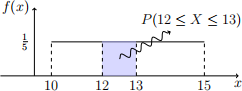
With this question, we will explore the probability distributions of continuous random vari-ables. Imagine a factory measures the length and weight of the light bulbs it produces. The length of the light bulbs, denoted by the random variable X, follows a uniform distribu-tion U[10, 15], meaning the lengths are evenly distributed between 10 cm and 15 cm. The weight of the light bulbs, denoted by the random variable Y , follows a normal distribution N(200, 102), meaning the weights have a mean of 200 grams and a standard deviation of 10 grams.

(a) Calculate analytically the probability that a randomly selected light bulb has a length between 12 cm and 13 cm. Note that the probability density function (PDF) of a uniform distribution is constant and defined as:

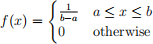
where a and b are the minimum and maximum values of the distribution. For this case, a = 10 and b = 15. The probability corresponds to the shaded area under the PDF curve between x = 12 and x = 13. To calculate it, use the formula:

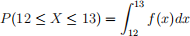
In other words, you need to calculate the shaded area shown below.

(b) Now, we will calculate the probability using a different method by approximating it. We will generate many random points between 10 and 15 and compute the proportion of points that fall between 12 and 13. This method is called a Monte Carlo simulation. Use the runif() function to sample 100000 points from a uniform distribution and approximate the probability that a randomly selected light bulb has a length between 12 cm and 13 cm. Compare the simulated probability with the analytical result. (Hint: Refer to the Hint file in Canvas.)

(c) Using the Monte Carlo simulation above, approximate the probability that a randomly selected light bulb has a length exactly equal to 12.5 cm under the uniform distribution. Briefly discuss the result.

(d) Calculate the probability that a randomly selected light bulb weighs between 190 grams and 210 grams. You do not need to perform integration. Recall the material from high school(!) and use the standard normal Z-table (easily available online). Note that if Y ∼ N(200, 102), the standardized random variable Z is defined as:

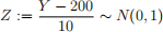
The probability can be expressed as:

where ϕ(y) represents the Bell-shaped standard normal distribution function.

(e) Use the rnorm() function to sample 100000 points from N(200, 102) and approximate the probability that a randomly selected light bulb weighs between 190 grams and 210 grams. Compare this simulated probability with the result obtained using the standard normal Z-table. (Hint: Refer to the Hint file in Canvas.)

7 Independent Research 1 (20 points)

One of the goals of this course is to prepare you to become a data scientist (broadly). To learn how to summarize, communicate, and estimate economic relationships and to evaluate policy, throughout this semester, you will practice this using the data and topic of your choice. The first step in research is often to pose a question and collect data.

(a) Find a specific dataset you would like to use and download it. The dataset should include two variables of your interest and at least one additional variable. How many observations and variables are there in the dataset? Where is the data from? Be clear about the data source. (In Canvas, I have provided some data sources you can use. You can, of course, change your topic and data later if needed. If you use confidential data, that’s fine, but please consult with me beforehand.)

Formulate your question. Please don’t be too ambitious. A simple question like ‘Would X affect Y?’ is enough. The only requirement is to be clear about the two variables you believe are related. For example, one example we discussed in class could be transformed into the question: ‘Would the level of education affect wages?’ Think about which areas of economics or other social sciences interest you. Find a dataset in that area and choose any two variables you think might be correlated. It is completely fine if you don’t find any significant result by the end of the semester–this is just for practice.

If this is not easy to do on your own, please don’t hesitate to consult with me.

(b) What is your research question? (Hypothesis)

(c) Does the dataset you have in (a) contain the variables needed to answer your question?

(d) What is your prediction on your research question?

(e) Provide any intuitive reasoning for your prediction in one to three sentences.