闪电代写 -代写CS作业_CS代写_Finance代写_Economic代写_Statistics代写_代码代做_IT代写_加急帮助

Hello, dear friend, you can consult us at any time if you have any questions, add WeChat: daixieit

EBU6503 Control Theory

Lab 2: Controller Design

– From Theory to Practice

Prerequisite

Install Matlab Simscape App

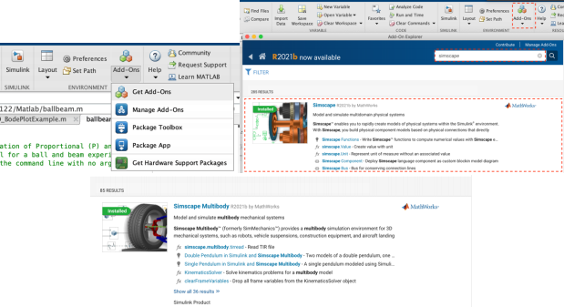
Please make sure the Simscape and Simscape Multibody add-on has been installed in Matlab as shown in the following pictures. You can find the information and install this add-on by clicking “Add-Ons” button.

Simscape™ enables you to rapidly create models of physical systems within the Simulink® environment. With Simscape, you build physical component models based on physical connections that directly integrate with block diagrams and other modelling paradigms. You model systems such as electric motors, bridge rectifiers, hydraulic actuators, and refrigeration systems, by assembling fundamental components into a schematic. Simscape Multibody™ provides a multibody simulation environment for 3D mechanical systems.

Introduction

A motor is an electromechanical component that produces a displacement output for a voltage input, i.e., a mechanical output generated by an electrical input. Applications for systems with electromechanical components are robot controls, sun and star trackers, and computer tape and disk-drive position controls.

In this lab, we will firstly derive the transfer function for one particular kind of electromechanical system, the armature-controlled DC servomotor. Then we will put this motor into a feedback control system and design a controller using root locus method (in Matlab) to make sure the transient and steady-state responses of the complete system meets the design requirements. Finally, we will verify the feedback control system design in Simulink.

Modelling

The schematic of the armature-controlled DC servomotor is shown in Figure 1 (a), and the transfer function we will derive is shown in Figure 1 (b) [1].

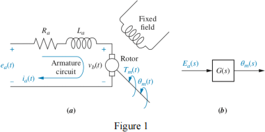
In Figure 1, a magnetic field is developed by stationary permanent magnets or a stationary electromagnet called the fixed field. A rotating circuit called the armature, through which current ! () flows, passes through this magnetic field at right angles and feels a force, = ! () , where is the magnetic field strength and is the length of the conductor. The resulting torque turns the rotor, the rotating member of the motor.

In this electromechanical system, the electric circuit can be modelled by applying Kirchoff's laws as we covered in Lecture 3: Mathematical Modelling, and the mechanical part of the system, the rotor, can be modelled by applying Newton’s laws for Rotational mechanical systems with the consideration of some electromagnetic effects.

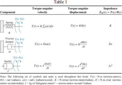
Rotational mechanical systems are handled the same way as translational mechanical systems (as you have learned in high school), except that torque replaces force, angular displacement replaces translational displacement and the term associated with the mass is replaced by inertia. Table 1 shows the components along with the relationships between torque and angular velocity, as well as angular displacement [1]. The values of K, D, and J are called spring constant, coefficient of viscous friction, and moment of inertia, respectively.

There is another phenomenon that occurs in the motor: A conductor moving at right angles to a magnetic field generates a voltage at the terminals of the conductor equal to = , where e is the voltage and v is the velocity of the conductor normal to the magnetic field. Since the current-carrying armature is rotating in a magnetic field, its voltage is proportional to speed. This voltage is called back electromotive force (back emf), which is given by

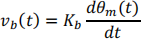
where " is a constant of proportionality called the back emf constant.

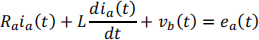
By applying Kirchhoff's voltage law and writing a loop equation around the armature circuit shown in Figure 1, we have

The torque developed by the motor is proportional to the armature current. So we have

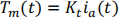
where # is the torque developed by the motor, and $ is a constant of proportionality, called the motor torque constant, which depends on the motor and magnetic field characteristics. In a consistent set of units, the value of $ is equal to the value of " . So let $ = " = .

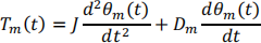
By apply Newton’s 2nd law and referring to Table 1 for the relationships between torque and angular velocity and inertia, we have

Question 1. Derive the transfer function of the armature-controlled DC servomotor, G(s), shown in Figure 1, where the angular velocity is considered the output and the armature voltage is considered the input, i.e., () = Θ̇ ()/! () .

[1.5 marks]

Design

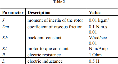
The physical parameters of the motor used in this lab are summarised in Table 2.

The most basic requirement of a motor system is that it should rotate at the desired speed. In this lab, the steady-state error of the motor angular velocity is desired to be less than 1%. Another performance requirement for the motor system is that it must accelerate to its steady-state speed as soon as it switches on. In this lab, the desired settling time is less than 1.5 seconds. Additionally, since a speed (angular velocity for the motor) faster than the reference speed may damage the equipment, we want an overshoot of less than 5% is desired for a step response.Design requirements

In summary, for a unit step command ( 1-rad/sec step reference) in motor speed, the control system's output should meet the following requirements.

1. Settling time less than 1.5 seconds.

2. Overshoot less than 5%.

3. Steady-state error less than 1%.

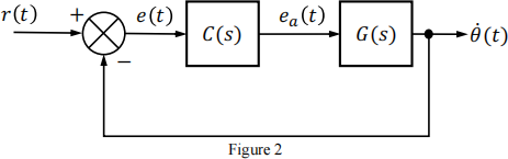
In order to meet the design requirement, a unity feedback control system with the structure shown below should be designed in this lab.

Control System Designer

The Control System Designer app lets you design single-input, single-output (SISO) controllers for feedback systems modelled in MATLAB® or Simulink® (requires Simulink Control Design™ software).

The documentation of the Control System Designer app can be found in “Control System Toolbox->Control System Design and Tuning->Classical Control Design->Control System Designer”

For design via root locus, the app is suggested to be launched using command “controlSystemDesigner('rlocus', plant_transfer_function)” .

Design via Gain Adjustment

Firstly, let us try to design the feedback control system shown in Figure 2 using root locus technique with only gain adjustment and investigate the system performance.

Question 2. Design a proportional-only compensator (gain adjustment) to meet the requirement for the transient response using Control System Designer. Find out if you can meet all the design requirement by only adjusting the gain in the forward path.