Section 1. Monte Carlo Statistical Methods

Question 1:  A-R sampling and M-H algorithm

In this question, our target density is:

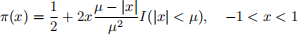
where I (.) is the indicator function, and 0 < µ < 1 is a parameter.

(a)  [ 5 marks] In your report, design an A-R sampling algorithm that generates random samples from π(x). Please find a suitable proposal density p(x) and an associated constant M for your algorithm, and show why p(x) is valid as a proposal density. Moreover, give the efficiency of your algorithm in the report.

In addition, in your R script please implement your algorithm by writing an R function called r.q1.ar, which should have the following features:

●  Arguments

–  mu:  the value of parameter µ in π(x)

–  n:  the number of random samples you want to generate

●  Return

–  an sequence of n random samples

Moreover, in the R script, use your function r.q1.ar to generate 2000 random numbers from π(x) to estimate the tail probability P(X > 0.8) for X ~ π(x) with µ = 0.5. Show your result in the report.

(b)  [ 6 marks] In your report, design an (independent) Metropolis-Hastings algorithm that generates random samples from π(x), using the same p(x) as you derived in (a) to be your (conditional) proposal density.

In addition, in your R script please implement your algorithm by writing an R function called r.q1.mh, which should have the following features:

●  Arguments

–  x0:  initial value of the chain

–  mu:  the value of parameter µ in π(x)

–  n:  the number of random samples you want to keep

–  m:  the number of burn-in random samples

●  Return

–  an sequence of n random samples

Moreover, in the R script, use your function r.q1.mh to generate 2000 random numbers from a Markov chain that admits π(x) as stationary distribution. Use those samples to estimate the tail probability P(X > 0.8) for X ~ π(x) with µ = 0.5, x0= 0.8, and m= 500. Show your results in the report.

(c)  [ 6 marks] Suppose we can find a sequence of proposal densities p1 (x), p2 (x), . . . with a sequence of positive numbers M1 , M2 , . . ., such that π(x) < Mipi (x) for _1 < x < 1 and i e N+ .  Now we can develope the following variation of A-R sampling:

Algorithm:  New A-R Sampling

In iteration i       ,  , . . .

1.  draw X = x from pi (x);

2.  draw Y = y from Unif(0,1);

3. If  accept X = x; otherwise reject.

Let p(x) and M  be the proposal density and constant you derived in  (a), respectively.   Consider

pi (x) = p(x) and 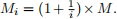 In you R script file, please implement above New A-R Sampling

probability P(X > 0.8) for X ~ π(x) with µ = 0.5. Show your results in the report.

In this case, which algorithm has a better efficiency, A-R Sampling or New A-R Sampling? Why? Write your answer in the report.

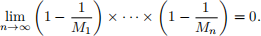
(d)  [ 6 marks] In your report, prove that the distribution of random samples generated by the New A-R Sampling algorithm is π(x) if

Hints:

(1) You can use existing random number generation functions in base R to help you generate samples from your proposal density p(x), such as runif, rnorm, rexp, etc.

(2)  For a random variable X generated from the A-R Sampling algorithm, note that

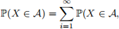 we rejeted at 1, . . . , (i _ 1)-th iterations and accepted X at i-th iteration).

Question 2:  Inverse Transformation Sampling and Gibbs Sampler

Let X = (X1 , X2 ) e R2  be a random vector with joint density function π(x) such that

where u is a 2-dimensional vector, Σ is a 2 x 2 matrix, a = (a1 , a2 ), and b = (b1 , b2 ) are all parameters. The notation x here means “is proportional to’ ’, i.e., f (x) x g(x) means f (x) = cg(x) for all x, where c is some fixed constant.

In this question, we consider a special case where a1  = a2  = a, b1  = b2  = b, µ = (0, 0), and

(a)  [ 5 marks] We know the conditional distribution for Xi IXj   = xj , denoted by N[a,b](µilj, σi(2)lj) with µilj  = ρxj  and σi(2)lj  = 1 _ ρ2 , has a density π(xi Ixj ) such that:

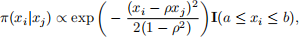
where i = 1, j = 2 or i = 2, j = 1. In your report, show that the inverse CDF of N[a,b](µilj, σi(2)lj) is

where Φ(.) is the CDF of N (0, 1). Based on this result, in your report, design an Inverse Transfor- mation Sampling algorithm that samples X1  conditional on X2  = x2 .

(b)  [8 marks] In your report, design a  Gibbs  sampler algorithm to generate random pairs  (X1 , X2 ) approximately from the target density π(x), with the initial value set to be X(0)  = (2.1, 2.3). Moreover, in your R script, implement this algorithm in a function called r.q2.gs, which should have the following features:

●  Arguments

–  n:  the number of random samples you want to keep

–  a:  the value of parameter a

–  b:  the value of parameter b

–  rho:  the value of parameter ρ

●  Return

–  a sequence of n random samples

In addition, apply your function r.q2.gs to generate 10000 random samples with a = 0, b = 2.5 and ρ = 0.7. Make the following plots in a 2 x 2 graph and show them in your report:

●  empirical marginal densities of X1  from your 10000 samples.

●  empirical marginal densities of X2  from your 10000 samples.

●  autocorrelation in the chain of X1

●  autocorrelation in the chain of X2

Hints:

(1) If you do not manage to prove the results in (a), you can still use them to proceed with algorithm-design and coding tasks in (a) and (b).

(2)  You can use any existing functions in base R, such as rnorm, dnorm, pnrom, qnorm, etc.

Question 3:  Iterated Monte Carlo

(a)  [ 5 marks] Suppose we want to sample n  =  kT random numbers/vectors approximately from the target density π(x), x e Rd . We can divide the n samples into T groups sequentially, i.e., denote the (tk _ k + 1)-th to tk-th samples as (X(1t) , . . . , X t)).

Instead of using a fixed proposal density, we now have a sequence of conditional proposal densities

qt)(x)  =  q(x Ixt - 1) )  available  for  t  =  1, 2, . . . , T  and  i  =  1, 2, . . . , k,  as  well  as  k  initial  values

(x  , . . . , x ).  In this way, we can do random number generation and update the proposal density

simultaneously.

Based on the above information, in your report, design a feasible new algorithm (let’s call it Iterated

MC) that does above job. Note that you cannot pose any further assumptions on qt)(x).

(b)  [9 marks] Suppose we want to generate random vectors from a bivariate mixture of Gaussians target density:

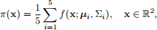
where f (x; u, Σ) denotes a bivariate joint normal distribution density with mean vector u and covariance matrix Σ .

In your report, apply the idea of your proposed Iterated MC to design a specific algorithm for this

problem.  The conditional proposal density is qt)(x) = f (x; xt - 1) , σ 2 I2 ), where I2  is the 2-dimensional

identity matrix.

Moreover, let

and

The initial X , . . . , X are just generated uniformly within the [_4, 4] x [_4, 4] square. In your R

script,  implement  above  algorithm  in  a  function  called  r.q3.imc ,  which  should  have  the  following

features:

●  Arguments

–  n:  the number of random samples you want to generate

–  k:  the number of samples in each group

–  sigma:  the value of σ in proposal density

●  Return

–  a n x 2 matrix of random samples, each row corresponding a sample

Consider k = 100 and T = 1000, σ = 20.  Use your r.q3.imc to generate n random samples, and estimate the mean of target density using the n samples.

Hints: The true value of the mean vector of x in (b) should be E(X) = (1.6, 1.4)T .

Section 2. Expectation-maximisation algorithm & bootstrapping

Question 1:  Mixture of Poisson Distributions

Let K be a positive integer, a Poisson mixture model assumes that each sample is generated from one of K

Poisson distributions. If the ith  observation Xi  is drawn from the kth  Poisson distribution with k e {1, ..., K}, we have

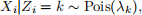
where λk  is the mean parameter of the kth  Poisson distribution.  The random variable Zi  indicates from which Poisson distribution Xi  is drawn, we assume

which means p(Zi  = k) = πk .

Consider the incomplete data scenario, where the variables Zi ’s are hidden. Let θ be the parameters of a Poisson mixture to be estimated. Specifically, θ = {π, λ}, where π = (π1 , ..., πK ) and λ = (λ1 , ..., λK ).

Follow parts (a)–(d) outlined below to write a program in R that uses the expectation-maximisation (EM) algorithm to find the maximum likelihood estimates (MLEs) of the parameters θ = {π, λ}.

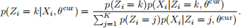
(a)  [ 6 marks] Recall that

Write a function poisMixEstep, which has the following features.

Arguments :

(1) piCur is a numeric vector of length K containing the current values of π .

(2)  lamCur is a numeric vector of length K containing the current values of λ .

(3) X is a numeric vector containing the values of X = {X1 , ..., XN }, i.e, the observed data.

Computation :

●  Calculate the conditional distribution p(Zi  = kIXi , θ cur ) for all k e {1, ..., K} and all i e {1, ..., N }.

Return :

●  A numeric matrix with N rows and K columns, where the entry in the ith  row and kth  column is the value for

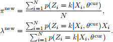
(b)  [4 marks] The expressions of θ new  = (πnew , λnew ) that optimize the function Q(θ, θcur ) is given by

Computation :

● Implement the EM algorithm to calculate the MLEs of π and λ of the Poisson mixture model. The number of Poisson distributions K in the mixture is determined by the the length of π . Thus, K is determined by the user.

●  You must use the functions you have created in parts  (a)—(c),  and also write additional R

commands to obtain a complete EM algorithm.

Return :

●  A list, where

– the first object is a numeric vector, containing the maximum likelihood estimates of π, and

– the second object is a numeric vector, containing the maximum likelihood estimates of λ .

Question 2:  Application of Inference under a Poisson Mixture Model using the EM Algoithm

You have met the playful British blue, Aristotle, in the Week 6 lab session.  In that lab session, we were analysing his diet patterns. To monitor his health status comprehensively, his owners are also interested in his activity patterns, which we will analyse in this question. The text file ‘activity.txt’ contains data on the number of times Aristotle headed out the house each week in the past 200 weeks.

According to his observant owners, Aristole’s activity patterns are mainly determined by his health status: 1) sick, 2) ‘healthy but inactive’ or 3) ‘healthy and active’.

However, his owners cannot always determine his health status by his appearance, so this factor is hidden. They can only observe the weekly frequency of him leaving the house.

Let Xi  be the number of times Aristotle leaves the house in week i, while Zi  is his health status that week.

For all i e {1, ..., 200}, we assume Xi  follows a Poisson mixture model (as described in Question 1) with K = 3.

Use your code in Question 1 to estimate the parameters θ of the Poisson mixture model.

You must use the following initial values for the parameters:

● π has the initial values (0.30, 0.45, 0.25).

●  λ has the initial values (1.5, 5.75, 15).

IMPORTANT: You must report your answer in the R script as comments!

Question 3:  Bootstrapping for the Coefficients of a Weighted Linear Regression

[ 10 marks]

Consider a dataset with a continuous response Y and only one covariate X.  We model this dataset by a weighted linear regression model:

where

●  yi  is the response of the ith  observation,

●  xi  is the value of covariate X of the ith  observation,

●  wi  is the positive weight of the ith  observation,

●  ei  is the error term of the ith  observation,

●  α is intercept,

●  β is coefficient of covariate X , and

●  σ 2  is the error variance.

The weighted least squares estimates of α and β are

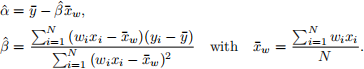
Write a function, called bootWLRegCoef, that calculates the standard errors of  and βˆ, using the bootstrap method and equations (7) and (8). The bootWLRegCoef function have the following features.

Arguments :

● x is a numeric vector representing the values of covariate X .

● y is a numeric vector representing the values of the response and has the same length as x.

● w is a numeric vector representing the values of the positive weights and has the same length as x.

● bootCount is a positive integer representing the number of bootstrap replicates to be used.

Computation :

●  Use the bootstrap method to calculate se() and se(βˆ), which are the standard errors of  and βˆ respectively.

Return :

●  A numeric vector, where

– the first element is the bootstrap estimate of se(), and

– the second element is the bootstrap estimate of se(βˆ).

Question 4

Imagine we have collected a dataset containing a covariate X and a response Y , assuming they are both continuous. We would like to model their relationship by a linear regression model, i.e.,

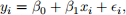
with ei  ~ Normal(0, σ2 ). The definition of the terms in equation (9) are outlined below.

●  yi  is the value of the response of the ith  observation.

●  xi  is the value of covariate X of the ith  observation.

●  ei  is the error term of the ith  observation.

●  β0  is the intercept of the linear regression.

●  β 1  is the regression coefficient of covariate X .

●  σ 2  is the error variance.

There was a problem with the instrument used to measure the value of X , and for each observation i, the true covariate value is within the interval [xi _ η, xi + η], where η is a positive real number.

Here, X is distributed according to a Gaussian mixture model, which have the following parameters.

●  K is the number of Gaussian distributions in the mixture model.

●  µ = (µ1 , ..., µK ), where µk  is the mean of the kth  Gaussian distribution.

●  σ = (σ1 , ..., σK ), where σk  is the standard deviation of the kth  Gaussian distribution.

● π = (π1 , ..., πK ), where πk  is the probability that an observation is generated from the kth  Gaussian distribution.

Hence, probability density function of X follows

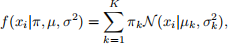
where X(.Iµk , σ k(2)) is the likelihood function of the kth  Gaussian distribution.

To account for the uncertainty associated with X, we consider the modified version of the MLEs of β0  and β 1 defined by equations (11)–(13) below.

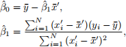
with

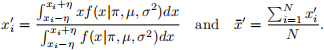
Write a function, called bootUncertReg, that calculates the standard errors of βˆ0  and βˆ1 , using the bootstrap method and equations (11)—(13). The bootUncertReg function have the following features.

Arguments :

● X is a numeric vector representing the values of covariate X .

● y is a numeric vector representing the values of the response and has the same length as X.

● mu is a numeric vector containing the means µ = (µ1 , ..., µK ) of the Gaussian mixture model.

●  sigma is a numeric vector containing the standard deviations σ = (σ1 , ..., σK ) of the Gaussian mixture model.

● pi is a numeric vector representing π = (π1 , ..., πK ).

●  eta is a positive numeric value representing η in equation (13).

● bootCount is a positive integer representing the number of bootstrap replicates to be used.

● tiCount is a positive integer representing the number of equal size sub-intervals for evaluating the integral in equation (13) using the trapezoidal rule.

Computation :

●  Use the bootstrap method to calculate se(βˆ0 ) and se(βˆ1 ), which are the standard errors of βˆ0  and βˆ1 respectively.

IMPORTANT: You must use the trapezoidal rule in ‘Section 2 Question 2 of Assignment 1’ to evaluate

the integral in equation (13) for your calculations to be considered correct.

Return :

●  A numeric vector, where