Hello, dear friend, you can consult us at any time if you have any questions, add WeChat: daixieit

18-698 / 42-632

Neural Signal Processing

Spring 2025

Problem Set 3

This problem set is due on Tuesday, March 11, 11:59pm.  Be sure to show your work and include all Matlab code and plots.

If you have questions, please post them on the Piazza Q&A webpage, rather than emailing the course staf. This will allow other students with the same question to see the response and any ensuing discussion.

Please submit your work as a single PDF file on Gradescope, which is linked from Canvas. When preparing your solutions, please complete each problem on a separate page.  Grade- scope will ask you select the pages that contain the solution to each problem.

Submissions can be written in LaTeX or they can be handwritten and photocopied using a scanner or smartphone camera.  Handwritten work should be clearly labeled and legible.

A probabilistic generative model for classification comprises class-conditional densities P(x | Ck) and class priors P(Ck), where x ∈ RD and k = 1, . . ., K.  We will consider three different generative models in this problem set:

i) Gaussian, shared covariance

x | Ck  ~ N (μk , Σ)

ii) Gaussian, class-specific covariance

x | Ck  ~ N (μk , Σk )

iii) Poisson

xi  | Ck  ~ Poisson(λki )

In iii), xi  is the ith element of the vector x, where i = 1, . . ., D.  This is called a naive Bayes model, since the xi  are independent conditioned on Ck .

1.  Maximum likelihood (ML) parameter estimation

In class, we derived the ML parameters for model i):

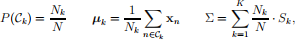
where

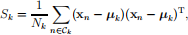
Nk  is the number of data points in class Ck , and N is the total number of data points in the data set.

For each of the models ii) and iii), find the ML parameters:

ii) (10 points)P(Ck ), μk , Σk

iii) (10 points) P(Ck ), λki

You can solve this problem for the two-class case, then generalize to K classes.

2.  (20 points) Decision boundaries

In class, we derived the decision boundary between class Ck  and class Cj  for model i):

where

For each of the models ii) and iii), derive the decision boundary between class Ck  and class Cj  and say whether it is linear.

3.  Simulated data

We will now apply the results of Problems 1 and 2 to simulated data.  The dataset can be found on Canvas under “Files → Data sets → ps3_simdata.mat” .

The following describes the data format.  The  .mat file has a single variable named trial, which is a structure of dimensions (20 data points)  × (3 classes).  The nth data point for the kth class is a two-dimensional vector trial(n,k) . x, where n = 1, . . . , 20 and k = 1, 2, 3.

To make the simulated data as realistic as possible, the data are non-negative integers, so one can think of them as spike counts. With this analogy, there are D = 2 neurons and K = 3 stimulus conditions.

Please follow steps (a)–(e) below for each of the three models. The result of this problem should be three separate plots, one for each model.  These plots will be similar in spirit to Figure 4.5 in PRML.

(a)  (6 points) Plot the data points in a two-dimensional space.  For classes k = 1, 2, 3, use a red ×, green +, and blue ◦ for each data point, respectively.  Then, set the axis limits of the plot to be between 0 and 20.  (Matlab tip:  call axis([0 20 0 20]))

(b)  (6 points) Find the ML model parameters using results from Problem 1.

(c)  (6 points) For each class, plot the ML mean using a solid dot of the appropriate color.

(d)  (6 points) For each class, plot the ML covariance using an ellipse of the appro- priate color.   This part only needs to be done for the  Gaussian models i) and ii).

(Matlab tip:  contour can be used to draw an iso-probability contour for each class. To aid interpretation, the contour should be drawn at the same probability level for each class.  For example, call contour(X, Y, Z, 0.007,‘r’).)

(e)  (6 points) Plot multi-class decision boundaries corresponding to the decision rule

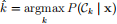                              (1)

and label each decision region with the appropriate class k. This can be done either by plotting appropriate segments of the pairwise decision boundaries derived in Problem 2, or by classifying a dense sampling of the two-dimensional data space. (Hint: You can check that you’ve done this properly by verifying that the decision boundaries pass through the intersection points of the contours drawn in part (d).)

4.  Real neural data

Neural prosthetic systems can be built based on classifying neural activity related to movement planning.  As described  in class, this is analogous to mapping patterns of neural activity to keys on a keyboard.

In this problem, we will apply the results of Problems  1 and 2 to real neural data. The neural data were recorded using  a  100-electrode array in premotor cortex of a macaque monkey1 .  The dataset can be found on Canvas under “Files → Data sets →

ps3_realdata.mat” .

The following describes the data format.  The .mat file has two variables:  train_trial contains the training data and test trial contains the test data.   Each variable is a structure of dimensions  (91 trials)  × (8 reaching angles).  Each structure contains spike trains recorded simultaneously  from 97 neurons while the monkey reached  91 times along each of 8 diferent reaching angles.

The spike train recorded from the ith neuron on the nth trial of the kth reaching angle is contained in train trial(n,k) . spikes(i,:),  where n =  1, . . . , 91, k =  1, . . . , 8, and i = 1, . . . , 97. A spike train is represented as a sequence of zeros and ones, where time is discretized in 1 ms steps.  A zero indicates that the neuron did not spike in the 1 ms bin, whereas a one indicates that the neuron spiked once in the 1 ms bin.  The structure test_trial has the same format as train_trial.

These spike trains were recorded while the monkey performed a delayed reaching task, as described in class.  Each spike train is 700 ms long  (and is thus represented by a 1 × 700 vector),  which comprises  a 200 ms baseline period  (before the reach target turned  on)  and a  500  ms  planning  period  (after  the  reach target  turned  on).   Be- cause it takes time for information about the reach target to arrive in premotor cortex (due to the time required for action potentials to propagage and for visual process- ing), we will ignore the first 150 ms of the planning period.  For this problem, we will take spike counts for each neuron within a single 200 ms bin start- ing 150 ms after the reach target turns on.  In other words, we will only use train trial(n,k) . spikes(i,351:550) and  test trial(n,k) . spikes(i,351:550) in this problem.

(a)  (10 points) Fit the  ML parameters of model i) to the training data  (91  × 8 data points).  Then, use these parameters to classify the test data (91  × 8 data points) according to the decision rule (1). What is the percent of test data points correctly classified?

(b)  (10 points) Repeat part (a) for model ii).  You should encounter a  Matlab warning when classifying the test data. Why did the Matlab warning occur?

(c)  (10 points) The answer to part (b) is a motivation for using a naive Bayes model.

Repeat part (a) for model iii).