3. Vibrations
Hello, dear friend, you can consult us at any time if you have any questions, add WeChat: daixieit
3. Vibrations
Introduction
In this experiment you will study the kinematics and dynamics of vibration, that is, the motion of a particle back and forth along a line. This study includes the definitions of amplitude, frequency, period and phase and the relationship between the kinetic and potential energy of the vibrating system. You will collect your data with a motion detector and a computer.
Theory
Why Study Vibrations?
Thus far in the first year physics lab you have studied linear motion. Certainly, examples of linear motion are to be seen all around us every day. But vibratory or oscillatory motion is actually the norm in nature. If the amplitude of a vibration is small then the motion is said to be simple harmonic. A pendulum swings with more-or-less simple harmonic motion. Water molecules on a pond bob up and down with simple harmonic motion. Electric and magnetic fields in radio waves vary with simple harmonic motion. Our hearts beat with simple harmonic motion. Certainly, the study of vibratory motion is as important as linear motion. This experiment and the experiment “Wave Motion” are complementary. Here we shall focus on the physics and mathematics of vibration as opposed to waves. But it should always be kept in mind that vibrations and waves are closely related.
Elasticity and Hooke’s Law
Some examples of simple harmonic motion depend for their existence on the elasticity of matter, for no object is perfectly rigid. All objects distort to some extent when acted on by an external force. If the object returns to its original shape when the force is removed then it is said to be elastic. The most common example of an elastic object is a spring, and the most common example of a simple harmonic oscillator is an object of mass m on the end of such a spring (Figure 3-1).
We shall show mathematically that the motion of the object in Figure 3-1 acted on by a Hooke’s Law force, or central force, is simple harmonic. When the spring is relaxed the object rests at some equilibrium position, say r0. If a force of magnitude F is applied to the object to stretch or compress the spring, then the spring responds with a force of the same magnitude acting in the opposite direction (a consequence of Newton’s Third Law).
This kind of force is also called a restoring force because the force attempts to restore the object to its equilibrium position. Robert Hooke (1635-1703), a contemporary of Isaac Newton, studied springs extensively in many experiments. He observed that the restoring force is directly proportional to the displacement as well as being in the opposite direction. If the displacement is small then the restoring force can be written in vector notation as
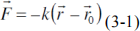
where k is a constant called the force constant of the spring (units newtons per meter, N.m-1). Eq[3-1] is known as Hooke’s Law in honor of its inventor. If the displacement is large enough then this linear relationship no longer holds.
If we displace the object in Figure 3-1 by a small amount and then release it, we should expect it to vibrate back and forth through its equilibrium position. If friction is negligibly small then the amplitude will be constant as well as the period. (The period is the elapsed time required for the object to complete one cycle or oscillation.) This is just what is meant by simple harmonic motion. The system as a whole (object and spring) is called a simple harmonic oscillator.
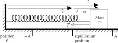
Figure 3-1. An object of mass m supported on a frictionless surface is shown here acted upon by a Hooke’s Law force.The object will execute simple harmonic motion. The displacement and force vectors are drawn in different head styles to emphasize their different natures.
A Real Simple Harmonic Oscillator
Before we get to the math of simple harmonic motion it is useful to preview the oscillator you will work with here. For reasons having to do with how the spring is made, the oscillator model of Figure 3-1 is impractical. (For the explanation see endnote 2.) The oscillator used here is a glider connected between two identical springs on an air track (Figure 3-2). This model differs from the model in Figure 3-1 in that two springs are used. Because of the two springs, we must replace the k in eq[3-1] with 2k.
The glider’s instantaneous position is continuously logged by a motion detector, the interface LabPro, and a computer as is done in the experiment “Linear Motion” . The same program, LoggerPro, is also used. The air track ensures that the glider moves with minimum friction. Recall that any vector pointing away from the detector is taken to have a positive sign, any vector pointing toward the detector is taken to have a negative sign.
The kinematics and dynamics ofa vibrating object can be developed as logically as is done for an object in linear motion. This we shall do in the next section.
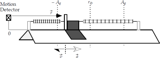
Figure 3-2. The harmonic oscillator used in this experiment is a glider connected between two springs on an air track. The glider is shown here at a clocktime when it is moving towards the origin (detector) before it has reached its maximum displacement to the left of the equilibrium position (closest point to the detector).
According to the sign conventions used by the detection system, the position of the glider is currently decreasing, its velocity is negative and decreasing, its acceleration is positive and increasing. Vectors are drawn here with different head styles to indicate their different natures.
The Equation of Motion
Our objective is to show that a Hooke’s Law force, eq[4-1], gives rise to the kind of motion described as simple harmonic. Putting eq[4-1] (where k is replaced by 2k) equal to mass times acceleration and rearranging we have the equation of motion
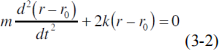
where we drop the vector notation for convenience. This is a second order homogeneous differential equation. It can be solved to get the position function.
Position
The solution of eq[4-2] is the position function r(t). You should be able to show by straight substitution that a solution is:
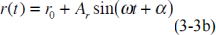
or
Where
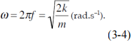
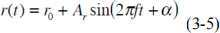
Writing eq[3-3b] in terms of linear frequency f we have
Thus r(t) is a sinusoidal function "offset" by the constant factor r0.
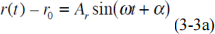
Eqs[3-3a and b] describe simple harmonic motion for the following reasons. r(t) is the instantaneous position of the glider measured with respect to the detector (Figure 3-2). The constant r0 is the glider’s equilibrium position (which you can set to zero in this experiment). The displacement r(t) – r0 is sinusoidal in time and therefore representative of a vibration. The factor Ar is the amplitude of the vibration (the glider's maximum displacement either side of the equilibrium position) and is a constant. ω is the angular frequency (in radians.s–1) and α (in radians) is the intrinsic phase angle of the source (the glider), which we shall call just the phase angle for short from now on. All these aspects define what is meant by a simple harmonic motion.
The Phase Angle
The detection system will enable you to investigate aspects of the glider’s motion down to the phase angle α . α tells you what the glider is doing at t = 0. Or in other words, its value is set by the glider’s position r(t) at t = 0. r(0) may have any value in principle; but in practice, its value depends on how you release the glider, or more precisely, on the glider’s position at the instant the detector starts logging data.
How α relates to the actual position versus clock time graphs that are obtained is explained in the series of drawings in Figure 3-3. Eq[3-5] is plotted for three phase angles: zero, +π/2 radians and – π/2 radians. You can see that the function with positive α may be regarded as shifted to the left with respect to the function with zero α whereas the function with negative α may be regarded as shifted to the right.
An actual position versus clock time graph logged by the software in this experiment is reproduced in Figure 3-4. You can see that the graph is consistent with Figure 3-3c to the degree that at t = 0 the displacement is negative and the velocity is positive (the glider is moving away from the detector). You can calculate α explicitly. Notice that at t = 0, r ≈ –0.048 m. Also ro ≈ 0, and Ar ≈ 0.180 m. Substituting these numbers into eq[3-5] we get
–0.048 = 0 + 0.180 sin (0 + α) ,
so that sin(α) = – 0.43636
and hence α = – 26° .
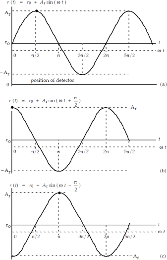
Figure 3-3. Three graphs of the function r(t)for three different values of the phase angle α: (a) zero, (b) + π/2 radians and (c) – π/2 radians. The function is “shifted” to the left for positive α and to the right for negative α. The dot on the curve may help you to visualize this. The position of the detector is shown along the bottom of (a). Thus in (a) the glider is moving through the equilibrium position at t = 0 in a direction away from the detector. In (b) the glider has reached a maximum displacement farthest from the detector and equilibrium at t = 0 and is on the point of reversing its movement. In (c) the glider has just reached a maximum displacement nearest to the detector at t = 0 and is on the point of reversing its direction.
Velocity
The velocity function is found by differentiating the position function, eq[4-5]:
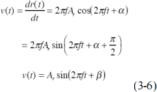
where we put β = α + π/2 to cast eq[3-6] in the form of eq[3-5] for comparison
purposes. Thus you can see that the velocity is a sinusoidal function of clocktime. The quantity Av = 2πfAr is the velocity amplitude. The angle β, the velocity phase angle, exceeds the position phase angle by π/2 radians. In the parlance of Figure 3- 3 the velocity is shifted to the left with respect to the position; thus the velocity leads the position by π/2 radians or 90° .
Acceleration
The acceleration function is found by differentiating the velocity function:
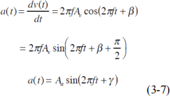
where we put γ = β + π/2 = α + π to cast eq[3-7] in the form of eq[3-5]. You can see that the acceleration is also a sinusoidal function of clocktime. The quantity Aa = 2πfAv is the acceleration amplitude. Using the same rationale as above, we can say that the acceleration leads the velocity by π/2 radians or leads the position by π radians. (Saying the acceleration leads the position by π radians is the same as saying the acceleration lags the position by π radians!) More output of the software in this experiment is reproduced in Figure 4-5 so you can confirm for yourself this discussion of math and phase.
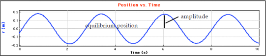
Figure 3-4. A position versus clocktime graph from LoggerPro showing the equilibrium position (zero) and amplitude of the simple harmonic oscillator. This graph is consistent with a negative phase angle, specifically of about –26° . Other LoggerPro graphs from this run are reproduced in Figure 3-5.
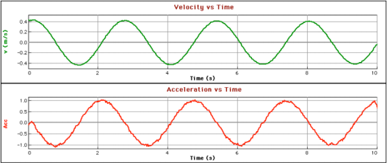
Figure 3-5. A typical output from LoggerPro (continuing from Figure 3-4). The velocity curve at the top leads (is displaced to the left from) the position curve (Figure 3-4) by π/2 radians and the acceleration leads (or lags) the position by π radians.
The Energy of a Vibrating System
Kinetic Energy
A simple harmonic oscillator can also be described in terms of energy. Since we have seen that position and velocity are sinusoidal functions, we expect the energy terms will be sinusoidal also. The kinetic energy of a mass m is given by the usual definition
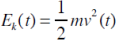
where we allow for time dependence. This expression becomes, when we substitute eq[3-6],
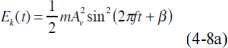
Or
where β = α + π/2. Thus we see that the kinetic energy function, involving the square of a cosine function, is a “double sinusoid” (meaning it has a frequency double that of a “single sinusoid”).
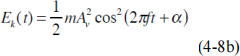
Potential Energy
The potential energy Ep is just the work required to stretch the spring by some displacement. This is given by the integral:
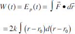
using eq[4-1] (allowing for a two spring model) and the fact that dr = d(r – ro). Thus:
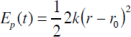
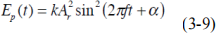
Or
Total Energy
Substituting eq[3-3a]. You should be able to show that the total energy E is
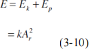
The total energy is therefore constant, or independent of time, provided friction is negligible. One of the objectives ofthis experiment is to study these aspects of energy.
2025-06-23