ECO00032M Investment and Portfolio Management 2020–21
Hello, dear friend, you can consult us at any time if you have any questions, add WeChat: daixieit
ECO00032M
MSc Degree Examinations 2020–21
Investment and Portfolio Management
Answer any THREE questions
1.
(a) [25 marks] [6.5] Consider a portfolio that offers an expected rate of return of 12% and a standard deviation of 18%. T-bills offer a risk-free 7% rate of return. Assume an investor with the utility function U = E(r) − 0.5 × Aσ2. What is the maximum level of risk aversion A for which she will prefer the risky portfolio to T-bills?
Answer: Since the return on T-bills is risk-free:
U(T − bills) = 0.07
The utility level for the risky portfolio is:
U = 0.12 − 0.5 × A × (0.18)2 = 0.12 − 0.0162 × A In order for the risky portfolio to be preferred to bills, the following must hold:
0.12 − 0.0162A > 0.07
A < 0.05/0.0162 = 3.09
A must be less than 3.09 for the risky portfolio to be preferred to bills.
(b) [25 marks] [6.12] Consider historical data showing that the average annual rate of return on the S&P 500 portfolio over the past 90 years has averaged roughly 8% more than the Treasury bill return and that the S&P 500 standard deviation has been about 20% per year. Assume these values are representative of investors’ expectations for future performance and that the current T-bill rate is 5%. An investor with the utility function U = E(r) − 0.5 × Aσ2 and the risk aversion coefficient A = 3 is considering three asset allocation choices: 20% − 80%, 40% − 60%
or 60% − 40% in Treasury bills and the S&P 500 portfolio, respectively.
Which portfolio should she choose?
Answer: Computing utility from U = E(r) − 0.5 × Aσ2 = E(r) − 1.5σ2, we arrive at the values in the column labeled U(A = 3) in the following table:
wBills rBills wSP E(rSP) E(rp)
rBills × wBills + E(rSP) × wSP
σp 0.2 × wSP
σ![]() U(A = 3)
U(A = 3)
|
0.05 0.05 |
0.1140 0.0980 0.0820 |
|
The investor should choose the portfolio 40% − 60%, since it yields the highest utility.
(c) [25 marks] [6.29] You estimate that a passive portfolio, that is, one invested in a risky portfolio that mimics the S&P 500 stock index, yields an expected rate of return of 13% with a standard deviation of 25%. You manage an active portfolio with expected return 18% and standard devia- tion 28%. The risk-free rate is 8%. Your client’s degree of risk aversion is A = 3.5. Assume the quadratic utility function: U = E(r) − 0.5 × Aσ2 .
i. If she chose to invest in the passive portfolio and the risk-free asset only, what proportion of her total wealth, y, would she invest in the index portfolio?
Answer: The formula for the optimal proportion to invest in the passive portfolio is:
E[rM] − rf
Aσ![]()
![]()
Substituting the following: E(rM ) = 13%; rf = 8%; σM = 25%; A = 3.5, yields:
0.13 − 0.08
y ∗ = = 0.2286 = 22.86%
ii. What is the fee (percentage of the investment in your fund, deducted at the end of the year) that you can charge to make the client indifferent between your fund and the passive strategy affected by his capital allocation decision (i.e., her choice of y)? Does it depend on the the client’s risk preferences portfolio?
Answer: The fee would reduce the reward-to-volatility ratio, i.e., the slope of the CAL. The client will be indifferent between my fund and the passive portfolio if the slope of the after-fee CAL and the CML are equal. Let f denote the fee:
Slope of CAL with fee
Slope of CML (no fee)
Setting these slopes equal we have:
0.10 − f
=
0.28
![]() =
=
0.18 − 0.08 − f 0.10 − f
= =
0.28 0.28
0.13 − 0.08
= = 0.20
0.25
0.20
0.044 = 4.4% per year
The fee that you can charge a client is the same regardless of the asset allocation mix of the client’s portfolio and thus it is independent of her risk preferences. You can charge a fee that will equate the reward-to-volatility ratio of your portfolio to that of your competition.
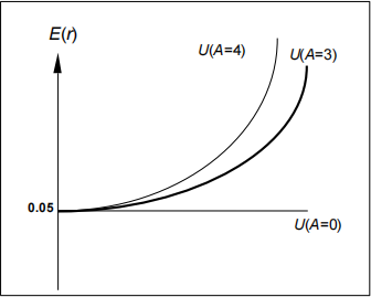
(d) [25 marks] [6.6-6.8] Draw the indifference curve in the expected return–standard deviation plane corresponding to a utility level of 0.05 for:
i. an investor with the utility function U = E(r) − 0.5 × Aσ2 with the risk aversion parameter A = 3;
ii. an investor with the utility function U = E(r) − 0.5 × Aσ2 with the risk aversion parameter A = 4;
iii. a risk-neutral investor.
Find the points corresponding to standard deviation, σ, equal to: 0.05, 0.10, 0.15 and 0.20. Answer: Points on the curve are derived by solving for E(r) in the following equation:
U = 0.05 = E(r) − 0.5 × Aσ2
E(r) = 0.05 + 0.5 × Aσ2
The values of E(r), given the values of σ2, are therefore:
σ σ2 E(r),A = 3 E(r),A = 4 E(r),A = 0
|
0.10 0.0100 0.15 0.0225 0.20 0.0400 |
0.0550 0.0700 0.0950 0.1300 |
0.0500 0.0500 0.0500 0.0500 |
2.
(a) [60 marks] [7.4-10] You are considering three mutual funds. The first is a stock fund, the second is a long-term government and corporate bond fund, and the third is a riskless T-bill money market fund that yields a rate of 8%. The probability distribution of the risky funds is as in the following table.
Expected Return Standard Deviation
Stock fund (S) 20% 30%
Bond fund (B) 12% 15%
The correlation between the fund returns is 0.10.
i. What is the expected return and standard deviation of the minimum-variance portfolio of the two risky funds?
ii. What are the expected return and standard deviation of the optimal risky (i.e. tangent) port- folio?
iii. You require that your portfolio yield an expected return of 14% and that it be efficient, on the best feasible Capital Allocation Line. What is the standard deviation of your portfolio? What is the proportion invested in the T-bill fund and each of the two risky funds?
iv. If you were to use only the two risky funds and still require an expected return of 14%, what would be the investment proportions of your portfolio?
v. Now suppose that the correlation between the two funds is − 1. Identify and explain an arbitrage opportunity in this case.
vi. Suppose that the stock and bond funds lie on the minimum-variance frontier, the market portfolio is the optimal risky portfolio from (ii) but the T-bill money market fund is not available. Find the weights of the market zero-beta portfolio.
Answer:
i. From the standard deviations and the correlation coefficient we generate the covariance matrix [note that Cov(rS .rB) = ρ × σS × σB]:
![]()
![]()
![]()
![]()
Bonds Stocks
Bonds 0.0225 0.0045
Stocks 0.0045 0.0900
The minimum-variance portfolio is computed as follows:
wMin (S) wMin (B)
σ![]() − Cov(rB ,rS) 0.0225 − 0.0045
− Cov(rB ,rS) 0.0225 − 0.0045
σ![]() + σ
+ σ![]() − 2Cov(rB ,rS) 0.0225 + 0.0900 − 0.0090
− 2Cov(rB ,rS) 0.0225 + 0.0900 − 0.0090
= 1 − wMin (S) = 1 − 0.1739 = 0.8261
The minimum-variance portfolio mean and standard deviation are:
E(rMin) = (0.1739 × .20) + (0.8261 × .12) = 0.1339 = 13.39%
σMin = [(0.173922 × 0.0900) + (0.826122 × 0.0225) + (2 × 0.1739 × 0.8261 × 0.0045)]1/2
= 0.1392 = 13.92%
ii. The proportion of the optimal risky portfolio invested in the stock fund is given by:
![]() S =
S =
=
|
[E(rS) − rf] × σ |
|
[E(rS) − rf] × σ |
= 0.4516
wS = 1 − w(B) = 1 − 0.4516 = 0.5484
The mean and standard deviation of the optimal risky portfolio are:
E(rp) = 0.4516 × 0.20 + 0.5484 × 0.12 = 0.1561 = 15.61%
σp = [(0.45162 × 0.0900) + (0.54842 × 0.0225) + (2 × 0.4516 × 0.5484 × 0.0045)]1/2
= 0.1654 = 16.54%
iii. If you require that your portfolio yield an expected return of 14%, then you can find the corresponding standard deviation from the optimal CAL. The equation for this CAL is:
E(rC) = rf + σC = 0.08 + 0.4601σC
If E(rC) is equal to 14%, then the standard deviation of the portfolio is:
0.14 − 0.08
σC = = 0.1304 = 13.04%
To find the proportion invested in the T-bill fund, remember that the mean of the complete portfolio (i.e., 14%) is an average of the T-bill rate and the optimal combination of stocks and bonds (P). Let y be the proportion invested in the portfolio P. The mean of any portfolio along the optimal CAL is:
E(rC) = (1 − y) × rf + y × E(rp) = 0.08 + y × (0.1561 − 0.08)
Setting E(rC) = 14% we find:
y 1 − y
= 0.7884
= 0.2119
![]()
To find the proportions invested in each of the funds, multiply 0.7884 times the respective proportions of stocks and bonds in the optimal risky portfolio:
Proportion of stocks in complete portfolio = 0.7884 × 0.4516 = 0.3560
Proportion of bonds in complete portfolio = 0.7884 × 0.5484 = 0.4323
iv. Using only the stock and bond funds to achieve a portfolio expected return of 14%, we must find the appropriate proportion in the stock fund (wS) and the appropriate proportion in the bond fund (wB = 1 − wS) as follows:
0.14 = 0.20 × wS + 0.12 × (1 − wS) = 0.12 + 0.08 × wS wS = 0.25
So the proportions are 25% invested in the stock fund and 75% in the bond fund. The stan- dard deviation of this portfolio will be:
σp = [(0.252 × 0.0900) + (0.752 × 0.0225) + (2 × 0.25 × 0.75 × 0.0045)]1/2
= 0.1413 = 14.13%
v. Since Stocks and Bonds are perfectly negatively correlated, a risk-free portfolio can be cre- ated. To find the proportions of this portfolio [with the proportion wS invested in Stocks and wB = (1 − wA) invested in Bonds], set the standard deviation equal to zero. With perfect negative correlation, the portfolio standard deviation is:
σp
0 wS
wB
= |wSσS − wBσB |
= wSσS − (1 − wS)σB
σB 0.15 1
σS + σB 0.30 + 0.15 3
2
= 1 − wS =
The expected rate of return for this risk-free portfolio is:
E(r) = (2/3 × 0.12) + (1/3 × 0.20) = 0.1467 = 14.67%
Thus, the arbitrage opportunity exist. We could borrow at the risk-free rate rf = 8% and invest in the risk-free portfolio yielding 14.67%. Such zero-investment strategy would yield 6.67% per period.
vi. The market zero-beta portfolio has zero correlation with the market portfolio and yields the same rate of return as the (shadow) risk-free asset.
0.08 = 0.20 × wS + 0.12 × (1 − wS) = 0.12 + 0.08 × wS
wS = −0.5
wB = 1.5
(b) [20 marks] [7.17] You run a fund invested in 30 equities drawn from several industries. One of your clients makes the following statement: “I trust your stock-picking ability and believe that you should invest my funds in your five best ideas. Why invest in 30 companies when you obviously have stronger opinions on a few of them?” Within the context of modern portfolio theory:
i. contrast the concepts of systematic risk and firm-specific risk, and give an example of each type of risk.
ii. provide a critique of the client’s suggestion. Discuss how both systematic and firm-specific risk change as the number of securities in a portfolio is increased.
[Word limit: 300]
Answer: Holding only the top, say, five best ideas would most likely result in the client holding a much more risky portfolio. The total risk of a portfolio, or portfolio variance, is the combination of systematic risk and firm-specific risk.
The systematic component depends on the sensitivity of the individual assets to market move- ments as measured by beta. Assuming the portfolio is well diversified, the number of assets will not affect the systematic risk component of portfolio variance. The portfolio beta depends on the individual security betas and the portfolio weights of those securities.
On the other hand, the components of firm-specific risk (sometimes called nonsystematic risk) are not perfectly positively correlated with each other and, as more assets are added to the portfolio, those additional assets tend to reduce portfolio risk. Hence, increasing the number of securities in a portfolio reduces firm-specific risk. For example, a patent expiration for one company would not affect the other securities in the portfolio. On the other hand, an increase in oil prices is likely to cause price reaction in different stocks across the market. For example, it is likely to cause a drop in the price of an airline stock but will likely result in an increase in the price of an energy stock. As the number of randomly selected securities increases, the total risk (variance) of the portfolio approaches its systematic variance.
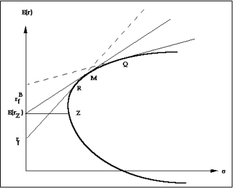
(c) [20 marks] [7.13] Assume that expected returns and standard deviations for all securities (in- cluding the risk-free rate for borrowing and lending) are known. Is it correct to assume that in this case all investors will hold the same optimal risky portfolio? Explain. [Word limit: 300]
Answer: No. If the borrowing and lending rates are not identical, then, depending on the tastes of the individuals (that is, the shape of their indifference curves), borrowers and lenders could have different optimal risky portfolios. The market portfolio will lie on the efficient frontier between portfolios R and Q in the following figure.
3. Consider the one-factor economy:
ri = E(ri) + βiF
where F is the systematic risk factor with zero mean and ei is the idiosyncratic risk. Assume that the risk-free asset exist. You have the following data for two well-diversified portfolios:
Portfolio Expected Return Beta
A 0.12 1.2
B 0.09 0.6
(a) [20 marks] What should be the risk-free rate in this economy? What is the return on the zero-beta
portfolio?
Answer: Notice that using well-diversified portfolios we can construct a risk-free portfolio with weights wA , 1 − wA with β = 0 (a zero-beta portfolio):
0
wA 1 − wA
= wAβA + (1 − wA)βB
= 1.2wA + 0.6(1 − wA)
= − 1
= 2
The rate of return on a well-diversified zero beta portfolio (rZ) is risk-free and thus, should be equal to the risk-free rate of return:
rZ = rf = − 1 × 0.12 + 2 × 0.09 = 0.06 = 6%
(b) [20 marks] What is the expected return on the factor-mimicking portfolio, E(rF)?
Answer: The factor mimicking portfolio has beta equal to one. Thus:
rF = E(rF) + F
We can construct a risk-free portfolio, as in (i), using the factor mimicking portfolio and, say, fund A. The weights, wA , 1 − wA, will be such that the beta of the portfolio is zero:
0
wA 1 − wA
= wAβA + (1 − wA)βF
= 1.2wA + 1(1 − wA)
= −5
= 6
Since this portfolio is risk-free, its return must be equal to the risk-free rate rf = 0.06:
0.06 = wArA + (1 − wA)rF
= −5[E(rA) + 1.2F] + 6[E(rF) + F]
= −5E(rA) + 6E(rF)
= −5 × 0.012 + 6E(rF)
E(rF) = 0.11 = 11%
(c) [20 marks] Derive the expected return-beta representation of this economy in terms of the risk premium on the factor-mimicking portfolio for all well-diversified portfolios. Explain carefully the steps in derivation.
Answer: Consider portfolio i with return:
ri = E(ri) + βiF
2022-01-08