EEEN30110 SIGNALS AND SYSTEMS
Hello, dear friend, you can consult us at any time if you have any questions, add WeChat: daixieit
SCHOOL OF ELECTRICAL & ELECTRONIC ENG.
EEEN30110 SIGNALS AND SYSTEMS
Laboratory SS_2
FOURIER THEORY
1. Objective:
To investigate the trigonometric Fourier series and Fourier analysis.
2. Background Information:
Before starting this laboratory generate some personalised digits. Let a, b, c be the last three digits of your student number. For example, if your student number is 19306127 then a = 1, b = 2 and c = 7. If any ofthese digits is 0 then add 1. For example, if your student number is 19306206 then a = 2, b = 1 and c = 6.
In this laboratory description document illustrative MATLAB commands are shown in purple. The problems which you are to solve are shown in blue. You must produce a report for this laboratory. This report will be graded and that grade will carry a weight of 28% when calculating your overall module grade. In this module the term “analytic expression” will be commonly used as the more technically correct term for “formula”. The number of grade steps which can be earned for each of the problems is given in the problem statement. As the number of problems is large this comprises a coarse grading scheme.
Consider the periodic continuous-time signal with period of 1 sec defined by
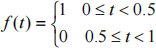
over one period. To generate the approximate Fourier coefficients ofthis periodic square-wave one must first generate a vector of samples uniformly spaced over one period ofthe signal. To achieve good speed of execution ofthe command it is better to ensure that the number of samples is a power of2. The following code generates 256 samples:
>> N = 256;
>> f = [ones(1,N/2) zeros(1,N/2)];
Now the command
>> FF = fft(f);
generates the sequence ofnumbers called Fn in the module notes. From the notes the Fourier coefficients are approximately  at least for small n that is to say for n small relative to N.
>> Fcoeff = FF/N;
The vector Fcoeff is now approximately the vector ofFourier coefficients. The first term is the zeroth coefficient, i.e. the DC or average value. One may determine this directly as follows:
>> Fcoeff(1)
ans =
0.5000
where the command Fcoeff(1) just picks out the first element ofvector Fcoeff. Of course it makes sense that the average value ofthe square-wave should be a half. The Fourier coefficients are complex numbers in general. In this case for example:
>> Fcoeff(2)
ans =
0.0039 - 0.3183i
Note that by default MATLAB uses i to denote the square root of - 1. It is not possible to plot complex data directly using the plot command in MATLAB. We commonly choose to plot the modulus ofthe coefficients. Consider the command
>> plot([0:31], abs(Fcoeff(1:32)), '. ')
which produces the following figure
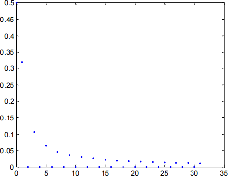
There are a number of observations to be made concerning this plot command. The command [0:31] generates the vector of numbers 0, 1, 2, 3, ... , 31. If the increment (or stride) in the definition of a vector is omitted it is assigned the default value of 1, so the command [0:31] and the command [0:1:31] generate the same vector. As noted in the table of basic functions the command abs determines the moduli of the elements of the vector, i.e. produces real data which the plot command can plot. The command Fcoeff(1:32) generates a sub-vector ofthe vector Fcoeff comprising the first 32 elements of Fcoeff, i.e. those elements with indices 1 through to 32. The reason for throwing away the rest of vector Fcoeff is that the approximation involved in determining the Fourier coefficients is only acceptably accurate for the first eighth or so ofthe coefficients. The additional term '.' in the plot command results in the plotting of the data using dots only, i.e. prevents the rather dubious default practice of joining up of the data points by line segments. From the plot we see that the zeroth coefficient has modulus 0.5 and that the second, fourth, sixth, etc coefficients are zero which is in agreement with the formula obtained in module notes. Of course as presented this plot is unacceptable since it has no axis labels. To reduce clutter the focus in this illustration is on how to actually produce the correct plot. For discussion of labels, title, caption and Figure number see previous laboratories SS_00 and SS_0, as well as module notes.
Note: in the problems which follow you are not asked to present the MATLAB code used in the solution of the problem, but rather the solution only, with exception ofrequirement to discuss choice of numerical parameter N.
Note: hand-written material is not acceptable. Equations must be produced with a proper equation editor.
3. Problems
The continuous time signal q(t) is periodic of period 2![]() sec. Over one period it is given by:
sec. Over one period it is given by:
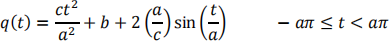
Problem 1: (0.75 grade step) Plot three successive cycles of the signal q(t).
Problem 2: (4 grade steps) Analytically determine the trigonometric Fourier series of the signal giving all of your calculations in detail.
Problem 3: (2 grade steps) Numerically determine the first thirteen Fourier coefficients of the signal. Your solution must offer justification/validation of your choice for critical parameter N in the numerical algorithm.
Note that the command fft assumes that first sample is at time t = 0. This is a complication here as the first value of t for which the formula is given does not equal 0.
A system with inputf and output g is described by the following differential equation
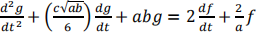
Problem 4: (0.5 grade step) Find the transfer function of the system and hence plot its magnitude response.
Problem 5: (2 grade steps) Using Fourier analysis analytically determine the trigonometric Fourier series of the output of this system when the input is the signal q(t) of Eq. (1) above, giving all of your calculations in detail.
Problem 6: (1.5 grade steps) Using the numerical result of problem 3 write out numerically
the first 25 terms ofthe trigonometric Fourier series of the output of system of Eq. (2) when the input is signal q(t) of Eq. (1). Compare this numerical solution with the analytical results of problem 5.
The voltage signal e(t) is periodic and has frequency 100a Hz. Over one period it is given by:
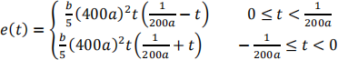
The signal is corrupted by a low amplitude mains hum, specifically the addition of 0.02sin(100![]() ).
).
Problem 7: (0.75 grade step) Plot three successive cycles ofthe corrupted signal. Offer evidence that this signal looks approximately like a sinusoid of amplitude b/5 and frequency 100a Hz, although corruption will be clearly visible if personal parameter b is small.
Problem 8: (4 grade steps) Analytically determine the trigonometric Fourier series of the corrupted signal, giving all of your calculations in detail.
Problem 9: (2 grade steps) Numerically determine the first thirteen Fourier coefficients of the uncorrupted signal e(t) and offer evidence that it is not a sinusoid. Your solution must offer justification/validation of your choice for critical parameter N in the numerical algorithm.
Problem 10: (2 grade steps) Using Fourier analysis analytically determine the trigonometric Fourier series ofthe output ofthe system of Eq. (2) when the input is the corrupted signal, i.e. e(t) of Eq. (3) with the additional mains hum, giving all of your calculations in detail.
Problem 11: (1.5 grade steps) Using the numerical result of problem 9 write out numerically the first 25 terms ofthe trigonometric Fourier series of the output of system of Eq. (2) when the input is the corrupted signal, i.e. e(t) of Eq. (3) with the additional mains hum. Compare this numerical solution with the analytical results of problem 10.
2022-01-05