EFIMM0091 Quantitative Methods for Accounting and Finance MOCK EXAM
Hello, dear friend, you can consult us at any time if you have any questions, add WeChat: daixieit
MOCK EXAM
Quantitative Methods for Accounting and Finance
EFIMM0091
Question 1 (10 marks)
Consider the following dataset:
![]()
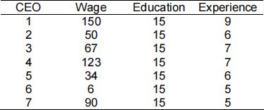
Is it possible to estimate the following regression equation?

Explain why it is/it is not possible to do it. (10 marks)
Question 2 (35 marks)
Petersen and Rajan (2002) document that the distance between firms and financial institutions is increasing over time. They find that the effect shows up as a steady trend throughout their sample, which spans from 1973 to 1993. Petersen and Rajan show that these results can be
explained by a greater use of information technology.
They estimate the following regression model:

where ln (1 + ![]()
![]()
![]()
![]()
![]() ) is the log of one plus the distance to the firm’s lender,
) is the log of one plus the distance to the firm’s lender, ![]()
![]()
![]() is the year in which the relationship with the lender started, and
is the year in which the relationship with the lender started, and ![]() include other control variables that might be correlated with distance, including
include other control variables that might be correlated with distance, including ![]()
![]()
![]()
![]()
![]()
![]()
![]()
![]() which is a dummy equal to one if the lender is a bank, and zero otherwise, and
which is a dummy equal to one if the lender is a bank, and zero otherwise, and ![]()
![]() ′
′![]()
![]() which is the age of the firm, among others.
which is the age of the firm, among others.
a) The following table presents the main result of the paper. Provide an interpretation of the coefficients presented below (![]()
![]()
![]() ,
, ![]()
![]()
![]()
![]()
![]()
![]() and
and ![]()
![]() ′
′![]()
![]() ), including the statistical and economic impact of these three explanatory variables presented in Column
), including the statistical and economic impact of these three explanatory variables presented in Column
(1) (15 marks).
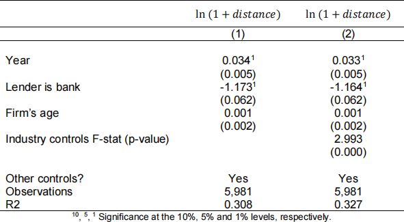
b) In robustness tests, the authors control for industry affiliation. They explain that “Including controls for the firm's industry (two-digit SIC) does increase the explanatory power of the model, but it does not change the coefficient on the year the relationship started”. Have these new controls potentially induced multicollinearity problems in the main variable of interest, Year? (10 marks).
c) Suppose the authors want to estimate following regression model:

![]()
where “Same city” is a dummy variable equal to one if the firm is located in the same city as the lender, and zero otherwise.
Explain how they could estimate that specification, and how they should interpret ![]() 1 (10 marks).
1 (10 marks).
Question 3 (25 marks)
The Capital Asset Pricing Model (CAPM) postulates that firm’s i expected risk premium (Ri−rf) is equal to that firm’s beta coefficient times the expected market risk premium (Rm−rf). If the CAPM holds, the intercept (alpha) is expected to be zero.
You have a dataset containing daily data on Exxon Mobile stock returns (Ri), the risk free rate (rf), and the market return (Rm) between January 3, 2011 until November 15, 2019.
a) Explain which type of model you could estimate to test the CAPM. Explain the nature of data, null hypothesis, and the regression equation (15 marks).
b) The Breusch-Godfrey test for autocorrelation yields the following results. What can you conclude from this table, and which are the potential consequences? (10 marks).

Question 4 (30 marks)
Khan, Serafeim and Yoon (2015) study the effect of corporate sustainability on firm performance. They find that firms with good ratings on material sustainability issues significantly outperform firms with poor ratings on these issues (material information is defined as presenting a substantial likelihood that the disclosure of the omitted fact would have been viewed by the reasonable investor as having significantly altered the total mix of information made available).
a) Read the following extract of the sample construction and explain the nature of the data (unit of analysis/frequency of data). (5 marks)
We use MSCI KLD as our source of sustainability data, the dataset most widely used by past studies. (…) It includes a large number of U.S. companies over a long period of time. In particular, between 1991 and 2000, it included approximately 650 companies; 2001– 2002, 1,100 companies; and 2003–2012, 3,000 companies. (…) The sample comprises 670 firms from the financial, 554 from the healthcare, 359 from the nonrenewable resources, 302 from the services, 388 from the technology and communications, and 123 from the transportation sector. In total, there are 2,396 unique firms and 14,388 unique firm years included in our sample.
b) The following table presents the main results of the paper. Compare the estimation methods in Columns (1) and (2) explaining the main differences, and advantages/disadvantages of each estimation method. (15 marks)
The dependent variable is two-year-ahead change in Return on Sales (ROS).
High Residual Materiality Index is an indicator variable for firms scoring at the top quintile of the residual materiality index.
High Residual Immateriality Index is an indicator variable for firms scoring at the top quintile of the residual immateriality index.
Firm controls include a set of time varying firm level controls such as Last Year’s Return, Size, Book-To-Market, Analyst Coverage and Leverage, among others.
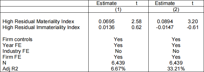
c) It has been suggested that Corporate culture (or attitude) towards Corporate Sustainability could be positively correlated with Materiality and Corporate Performance. How can this potentially omitted variable affect the results in Columns (1) and (2)? (10 marks)
2022-01-05