MTHM505J Data Science And Statistical Modelling In Space And Time – Ref/Def Assignment
Hello, dear friend, you can consult us at any time if you have any questions, add WeChat: daixieit
MTHM505J Data Science And Statistical Modelling In Space And Time – Ref/Def Assignment
This assignment consist of three sections. Section A consists of spatial modelling questions, Section B consists of time series modelling questions, and Section C is a project containing a report.
You should submit a pdf containing your answers to Section A, Section B, Section C (Questions 1-6) and your report for Section C Question 7.
For A, B and C (Q1-6) commented R code (and the outcomes/plots) should be part of your answers. For the report for Question C7 do not include R code in your report, please include it as an appendix.
The report for Question C7 should be no more than 6 pages (plus figures/tables/code appendix) and have the following sections:
● Introduction – explaining the rationale behind the analysis, e.g. what questions are you aiming to answer.
● Initial Data Analysis – provide the reader with graphical and numerical summaries that highlight any spatial and temporal patterns.
● Methods – describe the methods that you are going to use for your main analysis, highlighting why your choices are appropriate.
● Results – present the results of your analyses together with a clear narrative that will help the reader understand the results.
● Summary – summarise the key findings of your analysis, what were the answers to your questions?
● Bibliography - listing any papers and/or online sources that you reference in your report.
● Appendix – R Code.
A. Spatial modelling [100 marks]
You have just started work at an oceanographic consultancy. You are asked to interpolate a set of sea surface temperature data for one month in the Kuroshio off Japan onto a grid with a resolution of .5° in both the E and N directions. We are going to assume a flat Earth!
The data are in the file kuroshio.csv on ELE. An R program to read the data (readkuro.R) is also on ELE.
1. Produce numerical and graphical summaries of the data. Comment on your findings and highlight any potential outliers in the data. [10 marks]
2. Check for isotropy (the function variog4 in geoR may be useful). Do you need a trend in the model?
[20 marks]
3. Decide what spatial model you want to fit. You may want to try several and see which one fits best. Estimate the parameters of your chosen model by Maximum Likelihood and plot the expected value and variance for the estimate on the required grid. Validate your model. [35 marks]
4. Repeat 3 but use Bayesian methods. [25 marks]
5. Comment on the difference between the two methods of estimation. [10 marks]
B. Time series modelling [100 marks]
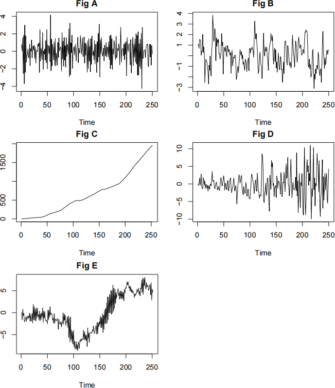
1. The figures labelled A to E show five time series whose defining equations are given below.
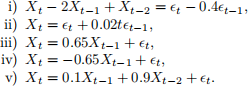
State, with reasons, which equation corresponds to which plot. [10 marks]
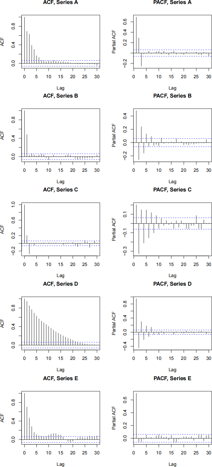
2. Suggest appropriate ARMA models for the five series (A, B, C, D, E) below, giving reasons for your choice in each case. [10 marks]
3. The data for this assignment are the measured strength of the overturning in the North Atlantic from moorings at 26N between April 2004 and March 2014, found in file overturning.csv.
a. Average the data to quarterly means. Produce numerical and graphical summaries of the averaged data, and comment on your findings and highlight any potential outliers. You might find it useful to convert the averaged data to a time series object ts(). [10 marks]
b. Fit an ARMA and an ARIMA model to the data. Choose the most appropriate model, and use this to predict the values for the six 3-month periods from April 2014 to September 2015. [30 marks]
c. Fit a DLM to the data (including both a trend and a seasonal component). Use your model to predict the values for April 2014 to September 2015. [30 marks]
d. Compare the results of parts b and c, and comment on any differences you may find. [10 marks]
C. Project [200 marks]
There are two data files from the National Oceanic and Atmospheric Administration (NOAA)’s National Centers for Environmental Information (NCEI). These are:
● (1) metadataCA.txt This file gives a number of sites, their elevations above sea level in feet, their geographic coordinates in latitude and longitude, and in the two right hand most columns, a reference point’s coordinates on the west coast of California linked to the site, that can be used to learn the site’s distance from the ocean.
● (2) MaxTempCalifornia.csv Maximum daily temperatures in degrees Celsius for those sites from Jan 1, 2012 to Dec 30, 2012.
Initial Data Analysis
1. Produce numerical and graphical summaries of the data from each site. Comment on your findings and highlight any potential outliers in the data. [10 marks]
2. Plot distributions of the data at each location. Comment on whether the data looks Normally distributed and, if not, suggest a suitable transformation. Perform an appropriate transformation and describe whether it now seems reasonable to assume that the data (at each location) is Normally distributed.
[10 marks]
3. Calculate monthly average (max) temperatures for each site. Plot the monthly averages for each location on the same plot and describe any temporal patterns that you see. [10 marks]
4. Perform a statistical analysis of whether there are differences in (max) temperatures at the different locations, and whether there are (statistically significant) differences between months. [20 marks]
Prediction
5. Using data only from San Francisco, develop a time series model and apply it to data from the other locations to predict maximum temperatures for all locations, for the 1st to 8th August 2012. Compare the predictions from your model with the observed measurements at all locations, and comment on how well your model fits the data, and how it performs at prediction. [30 marks]
6. Using only data from Napa, San Diego, Fresno, Santa Cruz, Ojai, Barstow, LA and CedarPark, develop a spatial model to predict maximum temperatures for San Francisco and Death Valley for 1st Jan 2012, together with associated measures of uncertainty (for the predictions). [40 marks]
Report
7. Perform an analysis of maximum temperatures over both space and time, and write a report summarising the spatial and temporal variation in maximum temperatures in California in 2012, detailing your choice of methods and the results. You may use the findings from Q1-6 as a precursor to your analysis for the report. As part of the report, you should create (at least one) map of temperatures and uncertainties based on predictions on a 10x10km grid. Your report should provide a clear commentary of the appropriateness of your chosen modelling approach(es) and any assumptions that you make, together with an assessment of how well any models you use perform in terms of model fit and predictive ability. [80 marks]
2021-12-31