Statistical Computing 2021

Programming language: For Section A you should use Tidyverse methods within the R programming language. Include Comments within your code. Foe sections B and C you can use either R or Python. Regardless of your    choice of language. It is essential that your answers are clear and well -written.

Submission structure: You should h a v e three separate reports corresponding to the three sections (A, B, C)of your work.  These folders should be entitled “user_SC _A”, “user_SC _B” and“user_SC_C”. Each of    these sub-folders should contain a report and a subfolder. The reports must clearly display your answers   to the corresponding section including both explanatory pros and snippets of code whereappropriate. The sub-folders should contain any data used to create the report and any supporting code(eg. .Rmd files        used to create your report). Hence, the subfolder “user_ SC _A” should contain afile entitled “user_SC       _A_Report” which displays all of your answers for Section A, the subfolder“user_SC_B” should contain a  file entitled “user_SC_B_Report” which displays all of your answers for Section B, and the subfolder  “user_SC_C” should contain a file entitled“user_SC_C_Report” which displays all of your answers for   Section C. The compiled reports“user_SC_A_Report”, “user_SC_B_Report” and “user_SC_C_Report”      can be either pdf or html documents. It is important that your approach to solving the questions is visible          within thesereports and you are encouraged to include pieces of clear and well-written code along with          explanatory proswithin the report itself.                                                                                                   Be careful to read each question in each section of the report.

Section A (30 marks)

In this part of your assessment you will perform a data wrangling task with some finance data.

Note that clarity is highly important. Be careful to make sure you clearly explain each step in your answer. You should also include comments within your code. In addition, make the structure of your answer clear through the use of headings. You should also make sure your code is clean by making careful use of Tidyverse methods.*

A.1

Begin by downloading the csv file available within the Assessment section within Blackboard entitled “fi- nance_data”.

Next load the “finance_data” csv file into R data frame called “finance_data_original”.How many rows and how many columns does this data frame have?

A.2

Generate a new data frame called “finance_data” which is a subset of the “finance_data_original” data frame with the same number of rows, but only six columns:

• The first column should be called “state_year_code” and correspond to the “state_year_code” column in the csv.

• The second column should be called “education_expenditure” and should correspond to the “De- tails.Education.Education.Total” column in the csv.

• The third column should  be called “health_expenditure”  and should correspond to the “De- tails.Health.Health.Total.Expenditure” column in the csv.

• The fourth column should  be called “transport_expenditure”  and should correspond to  the “De- tails.Transportation.Highways.Highways.Total.Expenditure” column in the csv.

• The fifth column should be called “totals_revenue” and should correspond to the “Totals.Revenue” column in the csv.

• The sixth column should be called “totals_expenditure” and should correspond to the “Totals.Expenditure” column in the csv.

Display a subset of the “finance_data” dataframe consisting of the first five rows and first three columns (“state_year_code”,“education_expenditure”,“health_expenditure”).

A.3

Create a new column within the “finance_data” data frame called “totals_savings” which is equal to the difference between revenue and the expenditure ie. the elements of the “totals_savings” column are equal to elements within

the “totals_revenue” minus the element within the “totals_expenditure” column, for each row. Your “finance_data” data frame should now have seven columns.

Display a subset of the “finance_data” dataframe consisting of the first three rows and the four columns “state_year_code”,“totals_revenue”,“totals_expenditure”,“totals_savings”.

A.4

The “state_year_code” column within your “finance_data” data frame contains both a state and a year in character format connected via a double underscore.

Divide the “state_year_code” column into two separate columns, a “state” column and a “year” column which replace the original “state_year_code” column.

Your “finance_data” data frame should now have eight columns.

Convert the states so that they appear with the first letter of each word in upper case and the remainder in lower case eg. we should see “New Hampshire” rather than “NEW HAMPSHIRE”. You may wish to use the function str_to_title().

Display a subset of the “finance_data” data frame consisting of the first three rows and the five columns “state”, “year”,“totals_revenue”,“totals_expenditure”,“totals_savings”.

A.5

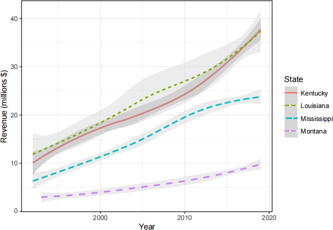
Generate a plot which displays the total revenue (“total_revenue”) as function of the year (“year”) for the following four states: Louisiana, Montana, Mississippi and Kentucky.

Display the revenue in terms of millions of dollars.

Your plot is expected to look as follows:

A.6

Create a function called get_decade() which takes as input a number and rounds that number down to the nearest multiple of 10. For example, the numbers 20, 21, 22, . . . , 29 would all be mapped to the output 20.

Use your get_decade() function to add a new column to the “finance_data” data frame called “decade” which should give the decade corresponding to the year column. For example, the decade of the years  1990,1991,. . . ,1998,1999 is 1990.

Your “finance_data” data frame should now have nine columns.

Which three states had the highest mean-average savings (“totals_savings”) over the decade starting 2000?

Note:

• When computing the average you should disregard any years in which the information is not available i.e. the average should be taken only over those years for which the savings entry is not an “NA”.

• You should aim to use a succinct Tidyverse type solution.

A.7

Next generate a summary data frame from the “finance_data” data frame called “alaska_summary” with the following properties:

Your summary data frame should correspond to rows associated with the state of Alaska. Your summary data frame should have three rows each corresponding to a decade from 1990 through to 2010 inclusive. Your data frame should also have seven columns:

(a) “decade” – the decade (1990, 2000, 2010)

(b) “ed_mn” – the mean of the education expenditure in Alaska for the corresponding decade   (c) “ed_md” – the median of the education expenditure in Alaska for the corresponding decade (d) “he_mn” – the mean of the health expenditure in Alaska for the corresponding decade        (e) “he_md” – the median of the health expenditure in Alaska for the corresponding decade      (f) “tr_mn” – the mean of the transport expenditure in Alaska for the corresponding decade     (g) “tr_md” – the median of the transport expenditure in Alaska for the corresponding decade

You should use Tidyverse methods to create your “alaska_summary” data frame.

Display the “alaska_summary” data frame.

A.8

Create a function called impute_by_median which takes as input a vector numerical values, which may include some “NA”s, and replaces any missing values (“NA”s) with the median over the vector.

Next generate a subset of your “finance_data” data frame called “idaho_2000” which contains all those rows in which the state column takes the value “Idaho” and the “decade” column takes the value “2000” and includes the columns “year”, “education_expenditure”, “health_expenditure”, “transport_expenditure”, “totals_revenue”, “totals_expenditure”, “totals_savings” (i.e. all columns except “state” and “decade”).

Now apply your “impute_by_median” data frame to create a new data frame called “idaho_2000_imputed” which is based on your existing “idaho_2000” data frame but with any missing values replaced with the corresponding me- dian value for the that column. That is, for each of the columns “education_expenditure”, “health_expenditure”, “transport_expenditure”, “totals_revenue”, “totals_expenditure”, “totals_savings” any missing values (given by “NA”) are replaced with the median over that column.

Display a subset of your “idaho_2000_imputed” data frame consisting of the first five rows and the four columns “year”, “health_expenditure”, “education_expenditure” and “totals_savings”.

Section B (30 marks)

B.1

In this question we consider a security system at a factory. A sensor is designed to make a sound if a person walks within one metre of the gate. However, the sensor is not perfectly reliable: It sometimes makes a sound when there is no one present, and sometimes fails to make a sound when someone is present.

For simplicity we will view the passage of time as being broken down into a series of phases lasting exactly one minute. For each minute, we let p0 denote the conditional probability that the sensor makes a sound if there is no person within one metre of the gate, during that minute. Moreover, for each minute, we let p1 denote the conditional probability that the sensor makes a sound at least once, if there is at least one person present, during that minute. Suppose also that the probability that at least one person walks within one metre of the gate over any given minute is q . Again, for simplicity, we assume that p0,p1,q ∈[0, 1] are all constant. Let ϕ denote the conditional probability that at least one person has passed within one metre of the gate during the current minute, given that the alarm has made a sound during that minute.

(a) Write a function called c_prob_person_given_alarm which gives ϕ as a function of p0,p1  and q . (b) Consider a setting in which p0 = 0.05, p1 = 0.95 and q = 0.1 . In this case, what is ϕ?

(c) Next consider a setting in which p0  = 0.05, p1  = 0.95 and generate a plot which shows ϕ as we vary q . That is, you should display a curve which has q along the horizontal axis and the corresponding value of ϕ along the vertical axis.

B.2

Suppose that α,β,γ ∈ [0, 1] with α+β  +γ ≤ 1 and let X be a discrete random variable with with distribution sup- ported on {0, 1, 2, 5}. Suppose that P (X = 1) = α, P (X = 2) = β , P (X = 5) = γ and P (X  {0, 1, 2, 5}) = 0.

(a) What is the probability mass function pX   : R → [0, 1] for X?

(b) Give an expression for the expectation of X in terms of α ,β,γ .

(c) Give an expression for the population variance of X in terms of α,β,γ .

Suppose X1, . . . , Xn    is a sample consisting of independent and identically  distributed  random variables  with P (Xi  = 1)  = α, P (Xi  = 2)  = β , P (Xi  = 5)  =  γ  and P (Xi   {0, 1, 2, 5})  = 0 for i  =  1, . . . , n.  Let X  := 1  Σn 

(d) Give an expression for the expectation of the random variable X in terms of α,β,γ .               (e) Give an expression for the population variance of the random variable X in terms of α,β,γ,n .

(f)  Create a function called sample_X_0125() which takes as inputs α, β, γ and n  and outputs a sample

X1, . . . , Xn   of  independent  copies  of X where  P (X  = 1)  =  α,  P (X  = 2)  =  β,  P (X  = 5)  =  γ  and P (X  {0, 1, 2, 5}) = 0.

(g) Suppose that α = 0.1, β = 0.2, γ = 0.3 . Use your function to generate a sample of size n = 100000

consisting of independent copies of X where P (X = 1) =  α,  P (X = 2)  =  β,  P (X = 5)  =  γ  and P (X / ∈0,{1, 2, 5 ) }=  0. What value do you observe for X?  What value do you observe for the sam- ple variance? Is this the type of result you expect? Explain your answer.

(h) Once again, take α = 0.1, β = 0.2, γ = 0.3 . Conduct a simulation study to explore the behavior of the

sample mean.  Your study should involve 10000 trials.  In each trial, you should set n = 100 and create a sample X1, . . . , Xn  of independent and identically distributed random variables with P (Xi   = 1)  =  α , P (Xi  = 2) = β, P (Xi  = 5) = γ  and P (Xi /  ,{1, 2, 5  )}= 0 for i = 1, . . . , n .  For each of the 10000 trials, compute the corresponding sample mean X based on X1, . . . , Xn .

(i) Generate a histogram plot which displays the behavior of the sample mean within your simulation study.

Use a bin width of 0.02. The height of each bar should correspond to the number of times the sample mean took on a value within the corresponding bin. 

(j) What is the numerical value of the expectation E(X) in your simulation study? What is the numerical value of the variance Var(X)? Give your answers to 4 decimal places.

Let fµ,σ   : R  → [0, ∞) be the probability density function of a Gaussian random variable with distribution N(µ, σ2), so that the population mean is µ and the population variance is σ2 .

(k)  Now append to your histogram plot an additional curve of the form x  ›→ 200 ·fµ,σ(x), which displays a

rescaled version of the probability density function of a Gaussian random variable with population mean µ  = E(X) and population variance σ2   = Var(X).  You may wish to consider your rescaled density x   ›→ 200 ·fµ,σ(x) displayed for a sequence of x-values between µ −4  ·σ and µ + 4σ in increments of 0.0001 . Make sure that the plot is well-presented and both the histogram and the rescaled density are clearly visible.

(l) Discuss the relationship between the histogram and the additional curve you observe. Can you explain what you observe?

B.3

In this question we shall use the exponential distribution to model time intervals between arrival times of birds at a bird feeder.

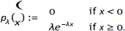
Let λ > 0 be a positive real number. An exponential random variable X with parameter λ is a continuous random variable with density pλ  : R → (0, ∞) defined by

(a) Give a formula for the the population mean and variance of an exponential random variable X with parameter

.

(b) Give a formula for the cumulative distribution function and the quantile function for exponential random

variables with parameter λ .

(c) Suppose that X1,    · ·,·X    n(is)  an i.i.d sample from the exponential distribution with an unknown parameter λ0  > 0. What is the maximum likelihood estimate MLE  for λ0?

(d) Conduct a simulation study to explore the behavior of the maximum likelihood estimator MLE   for λ0 on simulated data X1,  · · ·, Xn    generated using the exponential distribution.  Consider a setting in which λ0  = 0.01 and generate a plot of the mean squared error as a function of the sample size. You should consider a sample sizes between 5 and 1000 in increments of 5, and consider 100 trials per sample size. For each trial of each sample size generate a random sample1  X· ·, · , X n of the exponential distribution with parameter λ0   = 0.01, then compute the maximum likelihood estimate MLE   for λ0   based upon the corresponding sample. Display a plot of the mean square error of MLE  as an estimator for λ0  as a function of the sample size.

Now download the csv file entitled “birds_data_EMATM0061” from the Assessment section within Blackboard. The csv file contains synthetic data on arrival times for birds at a bird feeder, collected over a five week period. The species of bird and their arrival time are recorded.

Let’s model the sequence of time differences as independent and identically distributed random variables from an exponential distribution. More, precisely, let Y1, Y2, . . . , Yn+1  denote the sequence of arrival times in seconds. Construct a new sequence of random variables X1, . . . , Xn where Xi  = Yi+1 − Yi for each i = 1, . . . , n . Model the sequence of differences in arrival times X1, . . . , Xn  as independent and identically distributed exponential random variables.

(e) Compute and display the maximum likelihood estimate of the rate parameter MLE .

(f) Can you give a confidence interval for λ0  with a confidence level of 95%?

Note that clarity of presentation is highly important.  In addition, you should aim to demonstrate a depth of understanding.

1. Give a clear description of the supervised learning technique you will use. Explain how the training algorithm works and how new predictions are made on test data. Discuss what type of problems this method is appropriate for.

2. Choose a suitable data set to apply this model to and perform a train, validation, test split (some places to find data sets are described below). Be careful to ensure that your data set is appropriate for your chosen algorithm.  For example, if you have chosen to investigate a classification algorithm then your chosen data set must contain at least one categorical variable. Your data set for this task does not need to be large to obtain good results. The size of your data set should not exceed 100MB and you should aim to use a data set well within this limit. Your report should carefully give the source for your data. In addition describe your data set. How many features are there? How many examples? What type are each of the variables (eg. Categorical, ordinal, continuous, binary etc.?).

3. What is an appropriate metric for the performance of your model? Explore how the performance of your model varies on both the train and the validation data change as you vary the amount of training data used.

4. Explore how the performance of your model varies on both the train and the validation data change as you vary a hyperparameter.

5. Choose a hyper-parameter and report your performance based on the test data. Can you get a better understanding by using cross validation? Note that you will be graded on your understanding of the key concepts. It is far better to choose a simple hypothesis test and supervised learning algorithm, and apply sound statistical reasoning than to choose complex methods without properly demonstrating your understanding.

Alternative tasks

You could also choose an alternative task in which you explore a statistical method or methods which interest you.

A couple of elements to bear in mind here:

• Demonstrate a solid level of understanding of the technique or techiques you consider.

• Apply your chosen method or technique to a real data set. This data must be publicly available and should not exceed 100MB in size.

• Where appropriate, use simulated data to explore and demonstrate the properties of your chosen method.

• The subject of your report should be statistical methods or techniques and their performance and behaviour. Whilst you can consider techniques motivated by a particular application, the application itself should not become the focus of your report.

If you are unsure what to do for this section you are encouraged to discuss within the computer labs.

Note:

1. Do not complete and submit more than one of the above tasks. These are example tasks and you should only choose one. The goal here is to explore a topic in detail.

2. You will be graded on the level of understanding of the key concepts demonstrated within your report. With this in mind, it is far better to choose relatively simple methods, and apply sound statistical reasoning than to choose complex methods without properly demonstrating your understanding. You are welcome to include methods not covered within the lectures, provided that they are appropriate for the task at hand and that you are able to demonstrate a clear understanding of the methods used. A small number of additional marks will be given for more advanced methods, provided that a very strong level of understanding is displayed. However, the main focus here is a clear understanding and you should not sacrifice understanding for the sake of complexity. A clear understanding of the basic concepts is paramount.

3. You do not need to use large data sets. In Sections B and C you should not use data sets larger than 100MB. The total size of the data used within sections B and C cannot exceed 200MB. This is an upper bound. You should aim to use a data set well within this limit.

Data sets

There are a vast number of freely available data sets across the internet. Below is a few example sources. You are also welcome to use data sets from other sources. Any data you use should be freely available and accessible. The source of your data and the steps required to retrieve it should also be described within your main report.

You should also explain its structure eg. Number of rows and number of columns. You are encouraged to use tabular data throughout.

https://www.kdnuggets.com/datasets/index.html

https://r-dir.com/reference/datasets.html

http://archive.ics.uci.edu/ml/datasets.php

http://lib.stat.cmu.edu/datasets/

http://inforumweb.umd.edu/econdata/econdata.html

https://lionbridge.ai/datasets/the-50-best-free-datasets-for-machine-learning/

https://www.kaggle.com/

https://www.ukdataservice.ac.uk/

https://data.worldbank.org/

https://www.imf.org/en/Data