闪电代写 -代写CS作业_CS代写_Finance代写_Economic代写_Statistics代写_代码代做_IT代写_加急帮助

Hello, dear friend, you can consult us at any time if you have any questions, add WeChat: daixieit

COMS W4733: Computational Aspects of Robotics, Fall 2021

Homework 5

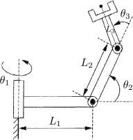
This assignment will focus on the nonplanar RRR manipulator shown below. For analytical ex- pressions, we recommend that you use the following shorthand whenever possible: s1 = sinθ1 , c23 = cos(θ2 + θ3), etc.

Problem 1: Forward Kinematics (20 points)

(a) Copy the figure and draw a set of coordinate frames consistent with DH convention. Place x0 along L1 and extend it rightward on the page.

(b) Using your frame assignment, derive the complete DH table in terms of the joint variables and link length parameters. There should be five columns and four rows.

(d) Describe the workspace that can be reached by the end effector if L1 = L2 = L3 .

Problem 2: Analytical Inverse Kinematics (15 points)

Suppose you are given a desired end effector position (xd,yd,zd). We would like to analytically solve for all possible joint configuration solutions q .

(a) Inspect the FK expressions for x and y and come up with a simple solution for θ1 in terms of xd and yd, assuming the manipulator is not singular.

(b) Once you have θ1, you can rearrange the x FK equation to contain unknowns in cos(θ2) and cos(θ2 + θ3) only. The FK for z should have a similar form with unknowns in sin(θ2) and sin(θ2 + θ3). Square and sum these equations and solve for θ3 .

Problem 3: Velocity Kinematics (20 points)

(a) Derive the linear velocity Jacobian Jv of the RRR manipulator by direct differentiation of the forward kinematics.

(b) Derive the angular velocity Jacobian Jω. Be sure to express the z axes of each successive frame with respect to frame 0.

(c) What is the rank of Jω? Which angular velocity component(s) (of the end effector) can be independently controlled, and which components are coupled?

(d) Compute and simplify an expression for the determinant of Jv. (You may wish to use a program for this.) Identify the arm singularity configurations of the manipulator and describe what these physically look like.

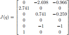
Problem 4: Inverse Velocity Kinematics (20 points)

Suppose that the RRR manipulator is in a configuration q such that its Jacobian is the following:

(a) Which single end effector velocity component generally yields no solution in the inverse velocity kinematics problem? Excluding the component you just identified, which pair(s) of end effector velocity components generally yield no solutions in the inverse velocity kinematics problem?

(b) Find either the exact or least squares solution to the IVK problem for the desired end effector velocities ξ1 = (x˙ , y˙ , z˙) = (1, 1, 1). Then do the same for ξ2 = (x˙ , z˙,ωy) = (1, 1, 1). Choose the minimum joint velocity norm solution if multiple solutions exist.

(c) Find the minimum joint velocity norm solution to the IVK problem for the desired end effector velocities ξ3 = (x˙ , y˙) = (1, 1), first using an identity weighting matrix and then using W = diag(10, 5, 1). Which components of the solution, if any, remain unchanged if a non-identity weighting matrix is used?

(d) Now suppose that we want the solution in (c) above to be as close as possible to q˙0 = (0.5, 0.5, 0.5), given W = I. Find a new solution to the IVK problem to satisfy this objec- tive. Which components of the solution, if any, remain unchanged?

Problem 5: Manipulability (15 points)

Let’s further analyze the linear velocity Jacobian (Jv, or the first three rows of J) of the RRR manipulator from Problem 4.

(a) Given a unit norm joint velocity vector, what is the largest possible end effector linear velocity? Please indicate both the magnitude and direction. Where does this velocity vector lie on the manipulability ellipsoid?

(b) Solve for the (unit norm) joint velocity vector that produces the end effector velocity that you found above. Where does this joint velocity appear in the singular value decomposition of Jv? Recall that the SVD decomposes 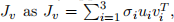where the ui are orthonormal left singular vectors and the vi are orthonormal right singular vectors of Jv .

(c) Suppose we are interested in end effector velocities orthogonal to the one you found in (a). What is the largest possible end effector velocity (magnitude and direction), and what is the corresponding unit norm joint velocity? Which joint(s) are actuated on the robot and in which direction(s) does the end effector move?

Problem 6: Iterative Inverse Kinematics (30 points)

The RRR manipulator has L1 = L2 = L3 = 1 and is currently in the configuration q = (0, 0, 0). We want to solve the inverse kinematics problem for the end effector to achieve the following pose:

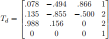
Note that an exact solution to this IK problem does not exist. Write a short program implementing both Newton’s method and gradient descent to find the joint configuration that will minimize the norm of the error (as defined in the lecture notes) between the desired and achieved pose. The two methods should only differ in a couple lines, but you will have to find suitable values for the damping constant in Newton’s method (if computation of a DLS pseudoinverse is needed) as well as the step size in gradient descent, so as to achieve convergence as quickly as possible.

For both experiments, report the values of any parameters that you tuned, the final error norm, and the solution to which the algorithms converge. Compare the two methods and comment on the following: rate of convergence, smoothness of the joint trajectories, stability of the solution, and algorithm sensitivity to parameters.

Problem 7: Learning Inverse Kinematics (30 points)

In this last problem, you will train a simple neural network to solve for the inverse position kine- matics of the RRR manipulator. For problems in which an analytical solution is not available or easy to use, a trained regressor may be more suitable than iterative methods, since prediction is effectively a constant-time operation. This is especially useful if joint configurations must be continuously solved for in real-time.

For full credit, you must perform the following three tasks:

• Use the forward kinematics (you may use L1 = L2 = L3 = 1) to generate a set of 1000 training data. You can uniformly sample joint configurations, keeping each θi between −π and π. You can then obtain the corresponding end effector (x,y,z) position for each joint configuration. Since we want to solve the inverse kinematics problem, the positions will form the inputs to the network and the joint configurations will form the outputs.

• Create a network model and train it using 80% of the data as training data. We recommend that you use Keras and keep the network simple; one nonlinear hidden layer with about 50 neurons should be sufficient (the input and output layers should each contain three neurons, matching the input and output sizes). Use mean squared error as your loss and plot both the (training) loss and validation loss versus epoch.

• Use your trained model to find a joint trajectory that would actuate the end effector to approximate the following trajectory:

You can copy and paste the following code into Python and simply call predict with your learned model. This matrix discretizes the trajectory into 500 points, each of which is stored in a row. Show plots of the resultant joint and end effector trajectories.

K = 500

traj = np.zeros((K,3))

traj[:,0] = 2*np.cos(np.linspace(0,2*np.pi,num=K))

traj[:,1] = 2*np.sin(np.linspace(0,2*np.pi,num=K))

traj[:,2] = np.sin(np.linspace(0,8*np.pi,num=K))

Please make sure that you have four plots altogether for the submission of this problem (in addition to your code).

Submission

You should have one document containing your solutions, responses, and figures for all written questions. At the end of the document, create an appendix with printouts of all code that you wrote or modified. Please tag your pages, including the relevant parts of the appendix. Submit both your document and code archive separately on Gradescope.