COMS W4733: Computational Aspects of Robotics, Fall 2021 Homework 4
Hello, dear friend, you can consult us at any time if you have any questions, add WeChat: daixieit
COMS W4733: Computational Aspects of Robotics, Fall 2021
Homework 4
Problem 1: Bayes Filter (20 points)
We have a robot in an infinitely long hallway located somewhere between x = − 1 and x = 1. We will use a uniform distribution over this domain as our prior belief distribution B(x0).
(a) The robot takes a noisy step in the positive x direction. Its motion model is given by a Gaussian distribution with unit variance: p(x1 | x0,u0) ∼ N(x0 + 0.5, 1). Compute the new belief distribution B′ (x1) after this step and generate a plot of the pdf. (The error function may be useful here.)
(b) The robot now picks up a sensor reading z1 that can only be read between x = −0.5 and x = 1.5. The observation model p(z1 | x1) is given by a uniform distribution over this domain. Compute the posterior belief distribution B(x1) after accounting for this sensor update and generate a plot of the pdf.
(c) Now suppose that we use a discrete Bayes filter instead. We discretize the state into four “cells” centered at x = −0.75, x = −0.25, x = 0.25, and x = 0.75. The probabilities of B(x0) are reweighted so that it is a proper discrete uniform distribution over these four state values. Compute the discretized distribution B′ (x1) given the same motion model as in part (a) (it is fine if the motion model is no longer a proper distribution).
(d) Combine the discretized B′ (x1) distribution above with the observation model in part (b) to compute the discretized posterior B(x1).
Problem 2: Homogeneous Transformations (15 points)
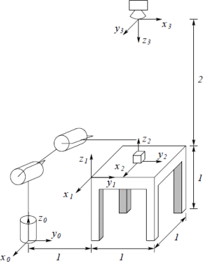
In the diagram below, a robot with base frame 0 is located 1 m away from a table, which is 1 m high and 1 m square. Frame 1 is rigidly attached to the table at the corner closest to the robot, and the two frames’ y axes are coincident. A cube is located at the center of the table, with frame 2 rigidly attached to the center of its bottom face. A camera is located 2 m directly above the center of the table, with frame 3 rigidly attached to it.
(a) Find the homogeneous transformations relating each frame to the previous one: A![]() , A
, A![]() , A
, A![]() .
.
(b) Suppose that the robot performs the following two actions. It pulls the table toward itself, translating the table and cube by −0.5 m along the y0 axis. It then rotates the cube 90 degrees clockwise about the z2 axis. Recompute each of the previous homogeneous transformations.
(c) Compute the composite transformation A![]() relating the camera frame to the robot frame. Would you get a different answer depending on whether you use the transformations from part (a) or part(b)? Describe the translational displacement and rotation between the two frames (the latter may be more sophisticated than a basic coordinate axis rotation).
relating the camera frame to the robot frame. Would you get a different answer depending on whether you use the transformations from part (a) or part(b)? Describe the translational displacement and rotation between the two frames (the latter may be more sophisticated than a basic coordinate axis rotation).
Problem 3: Forward Kinematics (15 points)
Consider the planar RPR manipulator shown below. Its joint variables are q = (θ1,d2,θ3), the link between the last joint and end effector has length a3, and a set of coordinate frames from the first joint to the end effector are shown. Note that the link between the two revolute joints has length equal to d2 .
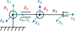
(a) Derive the complete DH table. There should be five columns (link, ai , αi , di , θi) and four rows (link, 1, 2, 3).
(b) Find the homogeneous transformations  corresponding to each row of the DH table.
(c) Find the composite forward kinematics  What are the position and orientation of the end effector as functions of the joint variables?
Problem 4: Differential-Drive Car Localization
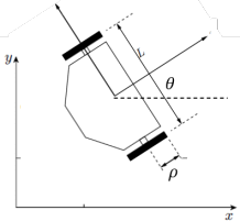
The differential-drive car shown below is a common mobile robot configuration. By independently controlling the velocities of its two wheels, the robot can translate and reorient on the plane. Its state vector is x = (x,y,θ), it has two inputs u = (u1,u2) corresponding to the angular velocities of its two wheels, ρ and L are fixed parameters, and ∆t is the timestep duration.
![]()
You will be implementing two different localization algorithms, one using the extended Kalman filter and one using the particle filter. The robot itself behaves according to models with nonlinear noise components and unknown to your estimators (it essentially moves around the plane in an imperfect circle). Instead, the filters will assume a standard nonlinear motion model with additive Gaussian noise xk = f(xk − 1 , uk) + wk, where
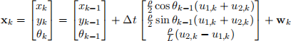
and wk ∼ N(0,Q). The vehicle has a range and bearing sensor, which measures its distance rk and angle ϕk from p fixed landmarks within the sensor’s maximum range. Again, these will have both nonlinear model and noise components, but your estimators will assume the standard model
zk = h(xk) + vk, where h = h1 ··· hp ,
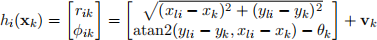
and vk ∼ N(0,Rk).
4.0: Code Description
We provide skeleton files based on localization examples from PythonRobotics. You will be filling out the necessary functions for EKF localization and particle filter localization. A description of the relevant variables and functions common to both files is provided below:
• WHEEL1 NOISE, WHEEL2 NOISE, and BEARING SENSOR NOISE are parameters describing the true robot model noise. Your estimators should not make reference to these.
• RHO and L are known physical parameters of the robot as shown on the above figure. MAX RANGE is the maximum range of the robot’s sensor. RFID is a list of known landmark positions.
• Q and R are covariance matrices used by your estimators.
• The remaining variables describe the time interval, total simulation time, number of particles in the particle filter, and the animation plot limits.
• The functions input, move, measure implement the “true” physics and behavior of the robot.
• The main function runs the simulation and displays an animation of the true robot trajectory in blue, estimated robot trajectory in red, and landmarks indicated by * symbols connected to the robot with black segments if sensed. A second plot shows the errors in the estimated state components at the end of the animation.
4.1: EKF Localization (15 points)
Recall that the EKF uses linearizations of the motion and observation models in Equations (1) and (2). Before you write any code, derive the Fk matrix by linearizing the motion model and show the result on your pdf. The linearization form of Hk is the same as the example from lecture.
Implement the EKF in ekf localization.py. The predict() function takes in the state mean, covariance, and velocity inputs. It computes and returns the predicted state mean and covariance.
The update() function takes in the state mean and covariance, as well as sensor measurements in the form of a p × 3 array. The first two columns contain an observed landmark’s sensed range and bearing, and the third column contains the landmark row index in RFID. From these you can compute and form the 2p innovation vector ![]() k, the 2p × 3 measurement linearization Hk, and the associated 2p × 2p measurement covariance matrix Rk . Rk contains p copies of the R matrix (for a single landmark measurement) along its diagonal blocks. You can then implement the update equations and return the updated state mean and covariance.
k, the 2p × 3 measurement linearization Hk, and the associated 2p × 2p measurement covariance matrix Rk . Rk contains p copies of the R matrix (for a single landmark measurement) along its diagonal blocks. You can then implement the update equations and return the updated state mean and covariance.
4.2: EKF Discussion (10 points)
Once you have implemented the above procedures, you can run the simulation loop in the main function, which will animate the robot’s true and predicted state trajectories. The state covariance is shown as a green dashed ellipse centered at the robot’s current location, although if your EKF is working properly the ellipse will generally be small enough to appear dot-sized. Answer each of the questions below using a few sentences each along with associated plots.
1. Run the full length of the simulation with the default parameters a few times. You should observe that the estimation is generally able to track the robot’s true state fairly well. Ex- plain any portions in which the errors increase by a noticeable amount and hypothesize why this occurs. Include two figures showing these observations, one with the last frame of the animation and the other with the plot of the state errors over time.
2. How are the covariance and accuracy of the state estimate affected if MAX RANGE is decreased to a value like 10? Show the resultant plots and explain how the number of sensed landmarks affects the accuracy of state estimation.
3. Now let’s explore the effect of starting with different initial estimates for the state mean and covariance (reset MAX RANGE to 18), which are set near the top of the main() function. First try increasing and decreasing P by several orders of magnitude and comment on whether you see any different initial behaviors. Then set the initial mean x est to something like (20, 20, 20) and show the resultant plots. Explain your observations.
4.3: Particle Filter Localization (15 points)
Now moving on to pf localization.py, the localization() procedure implements the main loop of the particle filter. It calls several helper functions: generate particles() to initialize (or
re-initialize) the filter, predict() and update() in each timestep, and resample() when sample weights become sufficiently low. Implement the last three functions. predict() returns a particle’s new state by sampling from the motion model in Equation (1). You can generate random Gaussian values to simulate wk .
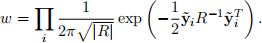
update() returns the weight for a given particle based on the measurement provided. As in the EKF, the measurement is a p × 3 array. Loop through each known landmark i in RFID. If you encounter either situation in which the predicted range rˆi ≤ MAX RANGE but landmark i is not in z, or conversely rˆi > MAX RANGE but it is in z, you can stop and immediately return the observation likelihood w = 0. Otherwise, compute the innovation ![]() i for landmark i. Assuming that
i for landmark i. Assuming that ![]() i is distributed according to a zero-mean Gaussian with covariance R and that each landmark measurement is mutually independent, the observation likelihood is given by
i is distributed according to a zero-mean Gaussian with covariance R and that each landmark measurement is mutually independent, the observation likelihood is given by
Finally, resample() performs the resampling process: given a current set of particles and their as- sociated weights, return a new set of particles generated by sampling from the provided information. This can be done very easily in Python using numpy.random.choice.
4.4: Particle Filter Discussion (10 points)
Once you have implemented the above procedures, you can run the simulation loop in the main function. The particles are represented by green dots, while the red trajectory represents the mean of their positions. Answer each of the questions below using a few sentences each along with associated plots.
1. Run the full length of the simulation with the default parameters a few times. You should observe that the estimation looks somewhat erratic with particles everywhere at the beginning, followed by a convergence to near the true robot state if the filter is working properly. Explain this particle behavior (and any other observations that you have) and include the two figures showing these observations.
2. How is the overall accuracy of the state estimate affected if MAX RANGE is decreased to a value like 10? Show the resultant plots and explain how the number of sensed landmarks affects the accuracy of state estimation.
3. Now let’s explore the effect of different numbers of particles (reset MAX RANGE to 20). Show what happens when we have only 10 or so particles. Why is it important to have a sufficiently large number of particles for accurate state estimation?
Submission
You should have one document containing your solutions, responses, and figures for all written questions. At the end of the document, create an appendix with printouts of all code that you wrote or modified for problem 4 (you should not include the entire files). Submit both your document and code archive separately on Gradescope.
2021-12-24