COMS W4733: Computational Aspects of Robotics, Fall 2021

Homework 3

Problem 1:  1-Dimensional Kalman Filter (15 points)

Consider a linear dynamical system in which the state, input, and output are all one-dimensional:

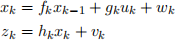
Everything is a scalar quantity, and the process and measurement noise are both distributed ac- cording to univariate Gaussian distributions: 

(a) Write out the complete set of Kalman filter equations for the estimates of the state mean  and variance p.  You should have equations for k|k − 1 , pk|k − 1 , k|k, and pk|k  in terms of k − 1|k − 1 , pk − 1|k − 1 , uk , zk, and the system parameters.  Please also expand the Kalman gain in your equations (do not leave in Kk).

(b) Examine the Kalman gain and the update equations that you derived.   Show the limiting behavior  of the  mean  and variance  updates when  1)  var(hkxk)  ≪  var(zk)  and when  2) var(hkxk) ≫ var(zk).

(c) The variance prediction and update equations depend solely on model parameters (f , g , h, q , r), not inputs or outputs. Suppose that all model parameters are constant over time. Derive a quadratic equation for the state variance pk|k in the limit as k → ∞, assuming that it converges to a fixed value. This should be an equation whose solution is p∞|∞ .

Problem 2: All Kinds of Noise (15 points)

The state evolution and measurement equations for a linear dynamical system are as follows:

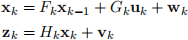
For this problem you may find it helpful to review the properties regarding transformations of Gaussian random vectors. You may omit details or steps that are identical to those in the lecture slides if you are able to specify exactly which simplifications or properties you are using.

(a) Suppose that the process noise wk is independently distributed according to a Gaussian distri- bution with nonzero mean, i.e. wk ∼ N(wk,Qk). Find the new prediction equations for k|k − 1 and Pk|k − 1, given k − 1|k − 1  and Pk − 1|k − 1 .

(b) Suppose that the process noise has zero mean, but that the inputs are independently distributed according to a Gaussian distribution: uk  ∼ N(uk,Uk). Find the new prediction equations for k|k − 1  and Pk|k − 1, given k − 1|k − 1  and Pk − 1|k − 1 .

(c) Suppose that the measurement noise vk  is independently distributed according to a Gaussian distribution with nonzero mean, i.e.  vk  ∼ N(vk,Rk).  Propose a change to the definition of the innovation y˜ to account for this. Briefly explain if the update equations will change or stay the same as a result.

Problem 3: Kalman Filter Simulation (20 points)

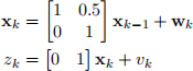
In this problem you will implement a Kalman filter for the simple robot moving along a straight line. Here we will assume that the robot does not take any inputs, so that its movement is all due

to its current velocity. We will also assume that the robot has a velocity sensor. Using timesteps of 0.5 seconds, the state and measurement equations are as follows:

As usual, we assume that wk  and vk  are distributed as zero-mean Gaussians, with covariance ma-

trix 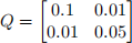 and variance r = 0.1, respectively.

We have provided you with a simple Python script, which should be fairly straightforward to un- derstand. Parameters are defined as above, and the robot’s initial state is x0 = (0.8, 2). Separately,

we also have the initial estimate of the state mean 0|0 = (2, 4) and covariance matrix 

Before starting this problem, run the script a few times. This moves the robot for 100 timesteps. Note that it is possible for the true state trajectory to vary quite drastically from one run to the next due to the inherent process noise.  As a sanity check, what happens when you manually set wk = 0?

(a) Implement the KF procedure, which runs one full iteration of the Kalman filter. That is, given k − 1|k − 1 , Pk − 1|k − 1, and zk, it should return k|k  and Pk|k. In your pdf submission, please copy and paste the code that you wrote verbatim. Run the full script at least two times and show the plots of the true and estimated state trajectories overlaid on each other.

(b) What happens to the state covariance, Kalman gain, and innovation covariance after a suitable number of iterations? Do this behavior and these results hold every time you run a simulation? Briefly explain your observations and the Kalman filter updates, despite the fact that the innovation itself continues to vary from one iteration to the next.

(c) The efficacy of the Kalman filter depends on having good estimates of the system model. Experiment with what happens when we drastically underestimate or overestimate the process noise. In the Kalman filter, you can scale Q by a very small value (or even 0!) and then a very large value (try at least 1000).  Show a couple representative state trajectory plots for each scenario and describe your observations.

(d) Repeat the above experiments with variations in the estimated measurement noise.  Perform similar scalings of r, show the state trajectory plots, and describe your observations.

Problem 4: Non-Euclidean RRT

Problem and Code Description

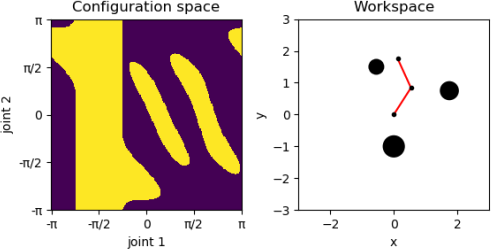
You will be implementing RRT construction for a RR robot arm. Remember that the configuration space of a RR arm is a torus, which is not Euclidean. In addition, it is often not trivial to construct representations of workspace obstacles in the configuration space. Below is an example of the two spaces side by side for an environment with three circular workspace obstacles.

We are providing the code file that generated the above figure, which you will also complete to generate RRTs on these C-spaces. Here is a brief rundown of the relevant portions of the code.

• At the top are several environment and RRT parameters. You may have to modify these as you develop and test your code. A class is also defined for a general n-link arm.

• Two utility functions are provided. detect collision is a collision detector for a given arm configuration. closest euclidean takes in two toroidal configurations q and q′  and returns q′′, a shifted version of q′. The L1 Euclidean distance between q and q′′ is equal to the toroidal distance between q and q′. This distance is also returned.

• You will be filling in the RRT methods  clear path, find qnew, find qnew greedy, and construct tree.

• The rest of the code includes a number of visualization functions.  You should not need to modify or invoke these yourself. Note that visualize spaces is commented out in the main function; this produced the above figure and is not used by the RRT. Remember that sampling methods do not need an explicit representation of the entire C-space.

4.1: Helper Functions (20 points)

Write the clear path and find qnew helper functions.  clear path is an incremental edge colli- sion detector.  Given two configurations q1 and q2 (represented as tuples), you should check each increment of EDGE INC on the segment between them, calling the detect collision method. Note that closest euclidean should be used to ensure that the correct, shorter segment is checked, instead of the longer one. The Boolean result should be returned when done.

find qnew takes in the RRT so far as well as a qrand configuration. It returns both qnear in the RRT and qnew  on the shorter segment between qnear  and qrand. The tree is represented as a dictionary, whose keys are nodes and values are the nodes’ parents.  To find the closest node in the RRT, it should suffice to iterate through tree.keys().  Again, closest euclidean should be used to ensure that the correct distances and segments are used. Assuming that qrand  is more than DELTA away from qnear , qnew  should lie exactly one DELTA away from qnear; otherwise, set qnew  to qrand .

4.2: RRT and Path Construction (15 points)

Write the construct tree function.  It should initialize the RRT as a dictionary with nodes as keys and parents as values, starting with {START: None} (we will build just one tree, so no tree at the goal).  Generate samples uniformly in [ −π,π] for both joint angles, and extend the tree until it contains either MAX NODES nodes or GOAL. If the latter condition is satisfied, a path can easily be constructed as a list of nodes by starting at GOAL and then tracing the parents back to START. Return the constructed tree and reversed path, or return an empty list for the latter if no path exists.

When you are finished, experiment with the parameters and run the main function for each of the two environments provided.  The C-space and workspace will pop up together, showing the constructed tree and the arm and obstacles.  The path will then be animated, with the C-space showing the nodes taken as red markers, and the workspace moving the arm to each corresponding configuration.  If a path was not found, the animation will not run and a failure message will be printed to the console.

For your parameters, use a DELTA of no more than 0.3.   Assuming a path exists, the value of MAX NODES is not as crucial as long as it is large enough, since tree construction should stop as soon as the goal is found. You should pick a suitable BIAS value, as well as an EDGE INC that is neither too small, slowing RRT construction, or too large, risking undetected collisions.

Include the final still images of the RRT and workspace for both environments in your writeup, and also save the animations to submit as videos. The videos should be saved in a publicly accessible location like Google Drive or YouTube, and links should be provided in your writeup (make sure to test these yourself!). You’ll also submit copies of these video files, described below.

4.3:  Greedy RRT Extension (15 points)

You should only start on this part once you’ve successfully implemented the basic RRT as de- scribed above.   Here you will implement the find qnew greedy method.   Start with a call to find qnew.  Then iteratively search outward along the segment between qnew  and qrand  in incre- ments of DELTA until you find an obstacle collision or until you reach qrand, at which point you should set qnew  = qrand.  The last usable increment is your final qnew, which should be returned along with the original qnear. (Here we will not return and add the intermediate nodes into the tree.)

Go back to construct tree and call the procedure you just implemented instead of the original version.   Show the results on the two environments once again.   Try changing the parameters if you are not able to find any paths; you can verify the correctness of your implementation by looking at the RRTs that are constructed, which should show tree branches of varying lengths. As in the previous part, save the final still images for both environments and provide links to the corresponding animations.