Computational Finance – HW 3
Hello, dear friend, you can consult us at any time if you have any questions, add WeChat: daixieit
Computational Finance – HW 3
1. A financial advising firm is experimenting with a new “probability fund” for its clients. When clients invest in this fund, they will be randomly invested in one of four assets whose returns are distributed normal, all with different expected returns and volatilities. The following table shows the probability of being invested in each asset along with their expected annual returns and volatilities:

• Pick the asset (1, 2, 3 or 4) at randomFix your random number generator seed at 1000 for reproducibility, then simulate 10,000 random returns from this probability fund. You can simulate one return in the following way, and you should vectorize this process or put it into a ‘for’ loop to generate 10,000 returns:
o Note: You can use the inverse transform method for generating discrete random variables that we learned in class or MATLAB’s randsample() function to generate your random assets.
• Simulate a random return using the randn() function and transform the value from standard normal to the proper distribution using the chosen asset’s expected return and volatility.
o Recall that a standard normal variable 
Now perform the following steps:
a. Plot and label a histogram of your 10,000 random returns. In just a sentence or two, describe the histogram.
b. Calculate and display the mean return you generated.
c. Using your knowledge of probability, calculate and display the theoretical mean for this fund. Comment on how it compares to your sample mean.
d. Calculate and display an estimate of the probability that the return on this fund will be negative based on your simulated returns.
e. Create a vector where each element i contains the mean for the first i elements of your sample. For instance, element 1 should be the first return from your sample, element 2 should be the mean of the first two returns, element 3 is the mean of the first 3 and so on, all the way up to element 10,000 as the mean of the entire sample.
f. Plot your vector of means from part d on the y-axis of a MATLAB figure, and then plot a red horizontal line whose y value is the theoretical mean return of the fund that you calculated in part c. (use the yline() function)
g. Describe what you see in your plot from part f and how it relates to the Law of Large Numbers.
2. The beta distribution is often used to represent the recovery rate after a corporate loan default (i.e., the amount recovered when the firm defaults). The CDF for the beta distribution unfortunately does not have a closed-form solution, so we cannot calculate a closed-form inverse CDF1 . However, the Kumaraswamy distribution is a distribution that we can use to approximate the beta, and it does have a closed-form CDF. The CDF for the Kumaraswamy is:
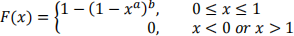
where a and b are “shape parameters” that determine the shape of the distribution.
The lgd.xlsx file contains data on N loan defaults, including a column containing the recovery rate for each loan (use MATLAB to find N when you need it).
a. Read in the Excel file. Use MATLAB’s betafit() function to estimate the a and b parameters for the best-fit beta distribution on the recovery rates. This function returns a vector where the first element is the estimated a and the second is the estimated b parameter.
b. Plot and label a histogram of the loan recovery rates, normalized by PDF (specified by ‘Normalization’,’pdf’ when you call the histogram function).
c. Use MATLAB’s betapdf() function to plot the PDF of beta using x values from 0 to 1 in increments of 0.01 on the histogram’s figure. The x values go on the x axis and the PDF values on the y axis. Does the histogram appear to fit the theoretical distribution well?
d. Simulate N Kumaraswamy-distributed numbers (using the inverse transform method) where a and b are the parameters you estimated in part
a. Plot the histogram of your simulated sample and a histogram of actual data in the same plot. Does your histogram match well?
Let’s use these simulated recovery rates to evaluate a potential loan with a 5% default probability and a 3% interest rate. In other words, if the loan does not default, the bank makes a 3% return on its investment. If it does default, the bank only recovers a fraction of its investment – your simulated recovery rate.
e. What’s the probability that the bank loses money?
f. If the bank is risk-neutral, should it make the loan?
2021-12-17