PHYS 305 - Optional* Problem Set 8
Hello, dear friend, you can consult us at any time if you have any questions, add WeChat: daixieit
PHYS 305 - Optional* Problem Set 8
Problem 1 - Richardson Extrapolation [10 points]
You don't need to code for this problem! Show your work.
Consider the function ![]() (x) =
(x) = ![]() exp(x).
exp(x).
![]() Compute the derivative of the function at x0 = 2 using the 2nd-order accurate centered difference
Compute the derivative of the function at x0 = 2 using the 2nd-order accurate centered difference
approximation to the derivative using Δx = 0.2, Δx = 0.1 and Δ![]() = 0.05. What is the relative error between the analytic (true) value of the derivative and the approximated value for each Δx? [2 points]
= 0.05. What is the relative error between the analytic (true) value of the derivative and the approximated value for each Δx? [2 points]
![]() Find the 3
Find the 3 ![]() (Δx2) approximations. What is the relative error between the analytic (true) value of the
(Δx2) approximations. What is the relative error between the analytic (true) value of the
derivative and these approximations? [2 points]
![]() Use Richardson extrapolation to derive an
Use Richardson extrapolation to derive an ![]() (Δx4) accurate representation of the derivative. What is the
(Δx4) accurate representation of the derivative. What is the
relative error between the analytic (true) value of the derivative and the ![]() (Δ
(Δ![]() 4) Richardson extrapolated value? Is it smaller than smallest
4) Richardson extrapolated value? Is it smaller than smallest ![]() (Δ
(Δ![]() 2) relative error? [2 points]
2) relative error? [2 points]
![]() Use Richardson extrapolation to derive an
Use Richardson extrapolation to derive an ![]() (Δx6) accurate representation of the derivative. What is the
(Δx6) accurate representation of the derivative. What is the
relative error between the analytic (true) value of the derivative and the ![]() (Δx6) Richardson extrapolated value? Is it smaller than the smallest relative error with the
(Δx6) Richardson extrapolated value? Is it smaller than the smallest relative error with the ![]() (Δ
(Δ![]() x4) Richardson extrapolated value? [2 points]
x4) Richardson extrapolated value? [2 points]
![]() What do your previous results imply about your abilitity to use Richardson extrapolation to obtain an error
What do your previous results imply about your abilitity to use Richardson extrapolation to obtain an error
estimate for your calculations at Δx = 0.2, Δx = 0.1 and Δx = 0.05. [2 points]
Problem 2 - Interpolation [10 points]
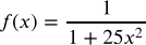
In this problem we will examine the Runge phenomenon, i.e., the problem of oscillation at the edges of an interval arising when using polynomial interpolation with polynomials ofhigh degree over a set of uniformly spaced points.
Consider the Runge function
and construct a grid of ![]() + 1 points in [
+ 1 points in [![]() ,
, ![]() ] = [− 1, 1],
] = [− 1, 1], ![]()
![]() =
= ![]() +
+ ![]() ∗ (
∗ (![]() −
− ![]() )/
)/![]() ,
, ![]() = 0, 1, …
= 0, 1, … ![]() , to store in the array xi , and the values of the function in the array yi=f(xi) to construct the Lagrange interpolantion polynomial.
, to store in the array xi , and the values of the function in the array yi=f(xi) to construct the Lagrange interpolantion polynomial.
In addition, construct an auxiliary grid ![]()
![]() = − 1. +
= − 1. + ![]() ∗ 2./
∗ 2./![]() ,
, ![]() = 0, 1, …
= 0, 1, … ![]() , with
, with ![]() = 100 onto which you will interpolate the function, using the degree
= 100 onto which you will interpolate the function, using the degree ![]() Lagrange interpolant.
Lagrange interpolant.
![]() Run your code for
Run your code for ![]() = 5, 9, 13, and make one plot of
= 5, 9, 13, and make one plot of ![]()
![]() vs
vs ![]()
![]() that contains all three cases and the exact
that contains all three cases and the exact
Runge function ![]() (
(![]() ) (four curves that should be clearly labeled). What do you notice near the edges of the interval? Do the interpolated values near the edges look like they are converging as
) (four curves that should be clearly labeled). What do you notice near the edges of the interval? Do the interpolated values near the edges look like they are converging as ![]() increases? [5 points]
increases? [5 points]
![]() One of the reasons for the Runge phenomenon is that the magnitude of the
One of the reasons for the Runge phenomenon is that the magnitude of the ![]() -th order derivatives of this
-th order derivatives of this
particular function grows quickly with increasing ![]() . The other reason lies in the choise of grid points (nodes) which are uniformly spaced. Instead of uniformly spaced grid points we can choose grid points that are more dense toward the edges of the interval. An example of such nodes are the Chebyshev nodes which are determined by
. The other reason lies in the choise of grid points (nodes) which are uniformly spaced. Instead of uniformly spaced grid points we can choose grid points that are more dense toward the edges of the interval. An example of such nodes are the Chebyshev nodes which are determined by
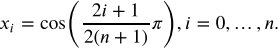
Repeat the previous step for ![]() = 5, 9, 13, but this time using the Chebyshev nodes which are not uniformly spaced. Does the choice of Chebyshev nodes mitigate the Runge phenomenon? [5 points]
= 5, 9, 13, but this time using the Chebyshev nodes which are not uniformly spaced. Does the choice of Chebyshev nodes mitigate the Runge phenomenon? [5 points]
Problem 3 - First-order Wave Equation [10 points]
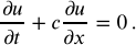
Consider the first-order wave equation in one spatial dimension (![]() ) with constant velocity
) with constant velocity ![]()
The analytic solution to this advection process is
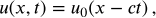
where ![]() 0(
0(![]() ) is the initial condition. In this problem, you will use this example to examine the performance of two finite-difference solution schemes.
) is the initial condition. In this problem, you will use this example to examine the performance of two finite-difference solution schemes.
Specifially, we solve this equation in the interval on the interval ![]() ∈ [0, 1] ,
∈ [0, 1] , ![]() ∈ [0, 0.25]
∈ [0, 0.25]![]()
![]()
![]() ℎc =1
ℎc =1 ![]()
![]()
![]()
![]()
![]()
![]() ℎ
ℎ![]()
![]()
![]()
![]()
![]()
![]()
![]()
![]()
![]()
![]()
![]()
![]()
![]()
![]()
![]()
![]()
![]()
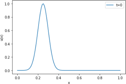
![]() 0(
0(![]() ) = exp(−200(
) = exp(−200(![]() − 0.25)2), ,$ which is illustratd below.
− 0.25)2), ,$ which is illustratd below.
For the numerical solution, we further impose Dirichlet Boundary condition ![]() (
(![]() = 0,
= 0, ![]() ) =
) = ![]() (
(![]() = 1,
= 1, ![]() ) = 0 .
) = 0 .
![]() Forward Euler, forward finite differentiation: Solve this problem numerically using the forward Euler
Forward Euler, forward finite differentiation: Solve this problem numerically using the forward Euler
method for the time integration and the first-order accurate forward finite difference scheme for the spatial derivative. Visualize the propagation of the wave by overplotting the spatial solution at different times. Discuss your result. [5 points]
![]() Forward Euler, backward finite difference differentiation: Solve this problem numerically using the
Forward Euler, backward finite difference differentiation: Solve this problem numerically using the
forward Euler method for the time integration and the first-order accurate backward finite difference scheme for the spatial derivative. Again visualize the propagation of the wave by overplotting the spatial solution at different times. Discuss your result. [5 points]

2021-12-11