Intro to Image Understanding (CSC420)

Assignment 4

General Instructions:

● You are allowed to work directly with one other person to discuss the questions. How- ever, the implementation and the report should be your own original work; i.e.  you should not submit identical documents or codes.  If you choose to work with someone else, write your teammate’s name on top of the first page of the report.

● Your submission should be in the form of an electronic report (PDF), with the answers to the specific questions (each question separately), and a presentation and discussion of your results. For this, please submit a file called report.pdf to MarkUs directly.

● Submit documented codes that you have written to generate your results separately. Please store all of those files in a folder called assignment4, zip the folder and then submit the file assignment4.zip to MarkUs.  You should include a README.txt file (inside the folder) which details how to run the submitted codes.

● Do not worry if you realize you made a mistake after submitting your zip file; you can submit multiple times on MarkUs.

● MarkUs has a file size limit. If your pdf or zip file IYou can try resizing or reducing the resolution of images in your report to reduce file size. If that doesn’t work, you can split

your report into multiple files (e.g. Reportp art1of3 .pdf, Reportp art2of3 .pdf, andReportp art3of3 .pdf)

Part I: Theoretical Problems (75 marks)

[Question 1] Camera Models (25 marks)

Assume a plane passing through point P→0  = [X0 , Y0 , Z0]T with normal n. The corresponding→  vanishing points for all the lines lying on this plane form a line, called the horizon.  In this question, you are asked to prove the existence of the horizon line by following the steps below:

1.  (15 marks) Find the pixel coordinates of the vanishing point corresponding to a line L, passing point P→0  and going along direction d→.

Hint:  = P→0 + td→ are the points on line L, and 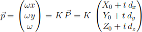 are pixel coordinates of the same line in the image, and  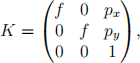where f is

the camera focal length and (px , py ) is the principal point.

2.  (10 marks) Prove the vanishing points of all the lines lying on the plane form a line.

Hint:  all the lines on the plane are perpendicular to the plane’s normal n; that is,→  n .→ d→ = 0, or nx dx + ny dy + nz dz  = 0

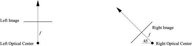
[Question 2] Epipolar Geometry (20 marks)

For a pair of rectified stereo cameras (i.e.  two identical parallel cameras, with a fixed dis- placement perpendicular to its optical axis) the epipolar lines on each image plane form a set of parallel lines, with the epipole at infinity. Now, let’s rotate the right camera for 45 degrees toward the left camera, as you see in the diagram below. For this stereo camera setup, show the epipolar lines and the epipole for each of the images planes.  Make sure to include your reasoning that justifies your answer.

[Question 3] Homogeneous Coordinates (30 marks)

Using the homogeneous coordinates:

1.  (15  marks)  (a) Show that the intersection of the 2D line l and lí  is the 2D point p = l Ⅹ lí .

2.  (15 marks) (b) Show that the line that goes through the 2D points p and pí is l = p Ⅹpí .

Part II: Implementation Tasks (75 marks)

[Question 4] Homography (55 marks)

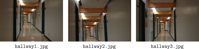
You are given three images hallway1.jpg, hallway2.jpg, hallway3.jpg which were shot with the same camera (i.e. same internal camera parameters), but held at slightly different positions/orientations (i.e. with different external parameters).

Consider the homographies H,

that map corresponding points of one image I to a second image I～, for three cases:

A. The right wall of I =hallway1.jpg to the right wall of I～=hallway2.jpg.

B. The right wall of I =hallway1.jpg to the right wall of I～=hallway3.jpg.

C. The floor of I～=hallway1.jpg to the floor of I～=hallway3.jpg.

For each of these three cases:

1.  (10 marks) Use a Data Cursor to select corresponding points by hand.  Select more than four pairs of points. (Four pairs will give a good fit for those points, but may give a poor fit for other points.) Also, avoid choosing three (or more) collinear points, since these do not provide independent information.  This is trickier for case C. Make two figures showing the gray-level images of I and I～with a colored square marking each of the selected points. You can convert the image I or I～to grey level using an RGB to Gray function (or the formula gray = 0.2989 Ⅹ R + 0.5870 Ⅹ G + 0.1140 Ⅹ B).

2.  (10 marks) Fit a homography H to the selected points.  Include the estimated H in the report, and describe its effect using words such as scale, shear, rotate, translate, if appropriate.   You are not allowed to use any homography estimation function in OpenCV or other similar packages.

3.  (10 marks) Make a figure showing the I～image with red squares that mark each of the selected (～x, y～), and green squares that mark the locations of the estimated (～x, y～), that is, use the homography to map the selected (x, y) to the (～x, y～) space.

4.  (20 marks) Make a figure showing a new image that is larger than the original one(s). The new image should be large enough that it contains the pixels of the I image as a subset, along with all the inverse mapped pixels of the I～image. The new image should be constructed as follows:

● RGB values are initialized to zero,

● The red channel of the new image must contain the rgb2gray values of the I image (for the appropriate pixel subset only );

● The blue and green channels of the new image must contain the rgb2gray values of the corresponding pixels (～x, y～) of I～  The correspondence is computed as follows: for each pixel (x, y) in the new image, use the homography H to map this pixel to the (～x, y～) domain (not forgetting to divide by the homogeneous coordinate), and round the value so you get an integer grid location. If this (～x, y～) location indeed lies within the domain of the I～image, then copy the rgb2gray’ed value from that I～(～x, y～) into the blue and green channel of pixel (x, y) in the new image.  (This amounts to an inverse mapping.)

If the homography is correct and if the surface were Lambertian* then correspond- ing points in the new image would have the same same values of R,G, and B and so the new image would appear be grey at these pixels.

● Based on your results, what can you conclude about the relative 3D positions and orientations of the camera ? Give only qualitative answers here. Also, What can you conclude about the surface reflectance of the right wall and floor, namely are they more or less Lambertian? Limit your discussion to a few sentences.

(5 marks) Along with your writeup, hand in a program that you used to solve the problem. You should have a switch statement that chooses between cases A, B, C.

*  Lambertian reflectance is the property that defines an ideal  “matte” or diffusely reflecting surface.  The apparent brightness of a Lambertian surface to an observer is the same regardless of the observer’s angle of view.  Unfinished wood exhibits roughly Lambertian reflectance, but wood finished with  a glossy coat of polyurethane  does not,  since the glossy coating creates specular highlights.  Specular reflection, or regular reflection, is the mirror-like reflection of waves, such as light, from a surface.  Reflections on still water are an example of specular reflection.

[Question 5] Mean Shift Tracking (20 marks)

In tutorial 10, we learnt about mean shift and cam shift tracking.  In this question we first attempt to evaluate the performance of mean shift tracking in a single case and will then implement a small variation of the standard mean shift tracking. For both parts you can use the attached short video KylianMbappe.mp4 or, alternatively, you can record and use a short (2-3 second) video of yourself.  You can use any OpenCV (or other) functions you want in this question.

1.  (10 marks) Performance Evaluation

● Use the Viola-Jones face detector to detect the face on the first frame of the video. The default detector can detect the face in the first frame of the attached video. If you record a video of yourself, make sure your face is visible and facing the camera on the first frame (and throughout the video) so the detector can detect your face on the first frame.

● Construct the hue histogram of the detected face on the first frame using appro- priate saturation and value thresholds for masking.  Use the constructed hue histogram and mean shift tracking to track the bounding box of the face over the length of the video (from frame #2 until the last frame). So far, this is similar to what we did in the tutorial.

● Also use the Viola-Jones face detector to detect the bounding box of the face in each video frame (from frame #2 until the last frame).

● Calculate the intersection over union (IoU) between the tracked bounding box and the Viola-Jones detected box in each frame.  Plot the IoU over time.  The x axis of the plot should be frame number (from 2 until the last frame) and the y axis should be the IoU on that frame.

● In your report, include a sample frame in which the IoU is large (e.g. over 50%) and another sample frame in which the IoU is low (e.g.  below 10%).  Draw the tracked and detected bounding boxes in each frame using different colours (and indicate which is which).

● Report the percentage of frames in which the IoU is larger than 50%.

● Look at the detected and tracked boxes at frames in which the IoU is small (< 10%) and report which (Viola-Jones detection or tracked bounding box) is correct more

often (we don’t need a number, just eyeball it). Very briefly (1-2 sentences) explain why that might be.

2.  (10 marks) Implement a Simple Variation

● In the examples in Tutorial 10 (and the previous part of this question) we used a hue histogram for mean shift tracking.  Here, we implement an alternative in which a histogram of gradient direction values is used instead.

● After converting to grayscale, use blurring and the Sobel operator to first gen- erate image gradients in the x and y directions (Ix  and Iy ).  You can then use cartToPolar  (with angleInDegrees=True) to get the gradient magnitude and angle at each frame. You can use 24 histogram bins and [0,360] (i.e. not [0,180]) directions.

● When constructing hue histograms, we thresholded saturation and value chan- nels to create a mask.  Here, you can threshold the gradient magnitude to create a mask.  For example, you can mask out pixels in the region of interest in which the gradient magnitude is less than 10% of the maximum gradient magnitude in the RoI.