Econ 113                                           Practice Problems for Final Review                                           Fall 2020

Examples of “conceptual” questions from midterm 1 material that are relevant for the final

1. The expected value ሺሻ of a discrete random variable X is ...:

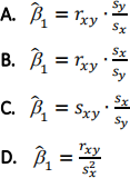
2. The OLS slope estimator from a simple linear regression of  on  can be written:

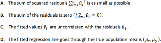
3. Which of the following is NOT a property (i.e., not something that is necessarily true, by construction) of the Ordinary Least Squares estimates from a simple linear regression of  on  :

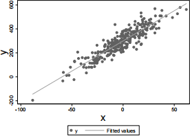
4. The figure below shows a scatterplot for a random sample of data on variables  and ,    along with the fitted ordinary least squares regression line from the regression of  on  .   The sample regression                function is given by   ൌ    ⃞   . The R2 for the regression is .833.

If one were to run a simple linear regression of x on y for this data (using the Stata command regress x y) this would result in:

A.   An R2 of 0.833, and a slope coefficient estimate of ‐ 5

B.   An R2 of 0.833, and a positive slope coefficient

C.   A different R2, and a slope coefficient estimate of ⅕ .

D.   A different R2, and a negative slope coefficient

5. When interpreting OLS estimates of a simple linear regression model, knowing the approximate      sampling distribution of the estimators ⃞ and ⃞  is important for (select the single most appropriate answer):

A.   Causal inference

B.    Statistical inference

C.    Neither causal nor statistical inference

6. When interpreting OLS estimates of a simple linear regression model, understanding the plausibility of the “zero conditional mean assumption” that ሺ|ሻ ൌ 0 is important for (select the single most      appropriate answer):

A.   Causal inference

B.    Statistical inference

C.    Neither causal nor statistical inference

Part 1.  The Stata output for Part 1 uses the data set wage2.dta.

a)  Refer to Model A:

     Why are only 857 observations used for to estimate this regression?

     Interpret the sign ofthe coefficient on the variable educXmeduc.  How does the return to     education vary with mother’s education? (Is an extra year of education worth more or less for individuals whose mothers were more highly educated)?

     Provide an alternative interpretation ofthe coefficient on educXmeduc.

b)  Refer to Model B.  Consider the model as a test for the presence of racial discrimination in   wages.  In other words, do black workers have lower wages, on average, that non-black        workers with similar qualifications such as levels of education, experience, and measures of knowledge and ability?

     Interpret the coefficient on black from this regression. What does the estimate suggest about the presence of discrimination?

     Is there statistical evidence of discrimination (i.e., is there a statistically significant racial wage gap among workers with similar qualifications?)

c)   Refer to Model C.

     Interpret the coefficient on the variable urban in model C1.

     Interpret the coefficient on the variable south in model C2.

     Explain why the coefficient on black changes in each model (compared to model B). What can you conclude about the correlations between the variable black and the      variables urban and south?

d)  Refer to Model D.

     What is the black-nonblack wage gap in the rest ofthe U.S. (non-South) holding constant everything in the model?

     Is the black-nonblack wage gap larger (in absolute value) in the South?

     By how much?

     Is the black-nonblack wage gap significantly different in the South compared to the rest ofthe U.S. (non-South)?  At what level of significance?

Part 2.  The Stata output for Part 2 uses data on 269 NBA basketball players, including average points scored  per game (points), experience (exper) and a dummy for whether they played basketball in college (coll). Note that guard and forward are dummy variables indicating the player’s position; center is the base category (i.e., there are 3 possible positions).  Circle the correct answer (each question has 1 answer):

1.    From the output following the command lincom guard‐forward  we can conclude:

A.    Controlling for experience and whether or not they played in college, the difference in average points scored by guards and forwards is statistically significant at a 10% level.

B.    Controlling for experience and whether or not they played in college, the difference in average points scored by guards and forwards is not statistically significant, even at a 10% level.

C.    Controlling for experience and whether or not they played in college, average points differs across positions (guard, forward, center) for at least one comparison, with significance at a 10% level.

D.    Controlling for experience and whether or not they played in college, there is no significant difference in average points across positions (guard, forward, center) even at a 10% level.

2.    From the output following the command test guard forward we can conclude:

A.    Controlling for experience and whether or not they played in college, the difference in average points scored by guards and forwards is statistically significant at a 10% level.

B.    Controlling for experience and whether or not they played in college, the difference in average points scored by guards and forwards is not statistically significant, even at a 10% level.

C.    Controlling for experience and whether or not they played in college, average points differs across positions (guard, forward, center) for at least one comparison, with significance at a 10% level.

D.    Controlling for experience and whether or not they played in college, there is no significant difference in average points across positions (guard, forward, center) even at a 10% level.

3.    If we were to re‐estimate the model using only 25% of the observations (selected at random), the standard errors on all of the coefficients would be approximately:

A.    4 times larger (i.e., 4X the original size)

B.    1.4 times larger (i.e., 1.4X the original size)

C.    2 times larger (i.e., 2X the original size)

D.   4 times smaller (i.e., 25% of the original size)

4.    If we were to re‐estimate the model using guard as the base category, the coefficient on center would be:

A.    ‐2.787

B.    4.658

C.    10.679

D.   ‐ 10.679

5.    If we were to re‐estimate the model using guard as the base category, the coefficient on forward would be:

A.    ‐0.916

B.    ‐2.787

C.    8.808

D.    2.787

6.    If we were to re‐estimate the model without using the vce(robust) option, which of the following would we expect to change (circle all that apply):

A.    The coefficients

B.    The standard errors

C.    The p‐values

D.   The confidence intervals

Part 3.  The Stata output for Part 3 uses data on Nielsen ratings for TV movies (movies produced for       television) from 1992. (This data is from an old MBA case study. Back in the “old days,” there were just three TV networks, and viewers mostly watched shows when they aired -- video recording was a pain!    Networks competed for “Nielsen ratings” which measured a show’s viewing audience when it aired.)

A.  Explain what each of the following commands does (see the bottom of the first page of output):

. gen abn = network==”ABN”

. gen factXstars = fact*stars

Refer to Models A & B

B.  A network executive is interested in knowing whether casting an additional star in a TV movie has a larger impact on ratings of a fact-based movie or a fictional one.  Which model is more useful for      answering this question? Explain.

C.  Calculate the effect of an additional star on the average rating of fact-based TV movies.

D.  Calculate the effect of an additional star on the average rating of fictional TV movies.

E.  Is the difference between the values corresponding to your answers to (C) and (D) statistically significant?

F.   Use Model B to calculate (i) the t-statistic and (ii) an approximate 95% Confidence Interval for the coefficient onfact. Is the coefficient statistically significant at a 5% significance level?

G.  Try answering the same questions as in F for the coefficient onfactXstars (assuming you only had the coefficient and standard errors).

Refer to Model C, which is a regression of ratings onfact and stars plus 8 dummy variables for 8 ofthe 9 months of the year (the sample includes only 9 months, as seen on the first page of output).

(Note: i.month in the regression tells Stata to automatically include a full set of dummy variables         named 2.month, 3.month, etc. for the categories in the variable month.  This shortcut can be used for any categorical variable with quantitative values. This is FYI; you do not need to know itfor thefinal.)

H.  Interpret the coefficient onfact from Model C.

I.    In which month are average ratings of TV movies highest, conditional on the type of move and number of stars?  In which month are average ratings the lowest?

J.   Do differences across months explain a significant share ofthe overall variation in the ratings of TV movies in this sample? How do you know?

K.  How, if at all, would your answer to J change ifDecember (month 12) were used as the base category in the regression instead of January (month 1)?

L.  Refer to Model D.  Write a brief explanation ofthe command test abn cbc (after the regression), and interpret the result.

Part 4.  The Stata output for Part 4 is an analysis of data on High School GPA.  The data include                 information obtained from a survey of 12,556 eleventh grade students who attend one of 88 randomly sampled high schools.

The variables include:

     drunk = 1 if the student has gotten drunk at least one time in the past year (and 0 otherwise)

     age is the student’s age in years

     twoprnthh = 1 if the student lives in a household with two parents (and 0 otherwise)

     male = 1 if the student is male (and 0 if female)

     schlcode is a categorial variable that indicates which high school the student attends.

A.   A researcher hypothesizes that one factor causing average high school GPA to be lower among boys than girls is that boys are more likely than girls to get drunk.  The researcher estimates      Model B, adding the variable drunk to Model A, and concludes that the results are consistent   with the hypothesis.  Explain briefly, using the omitted variables bias formula.

B.   The researcher now wants to know whether the effect of getting drunk on GPA differs for girls and boys, and estimates Model C.  What conclusion can be drawn from these results?

C.   Still referring to the results from Model C, calculate the difference in predicted GPA between   boys who have been drunk in the past year and boys who have not (holding constant their age and household structure).  (I.e., what is the partial effect on GPA of being drunk, for boys?)

D.   Suppose that the researchers added a set of school “fixed effects” (i.e., a dummy variable for  each of 87 out of the 88 schools in the data) to the regression model.  Briefly explain how this would affect the interpretation of the estimated coefficients on the other variables.

E.    Which of the following could still be part of the error term in the model with school fixed effects.  In other words, what is NOT held constant? (circle all that apply):

(i)   The training of the guidance counselors at the student’s school. (ii)  The difficulty of the student’s courses.

(iii) The school’s dropout rate in the previous year.

(iv) The fraction of a student’s close friends who skipped school in the past year.

(v)  The school’s average class size.

F.    Suppose that when the researcher added the school dummy variables to the model, the R‐          squared increased to .2697 (from .0599 in Model C). The research also performed and F‐test for the joint significance of the school dummy variables and obtained p=.002.  Interpret the results  of the F‐test in terms of the model’s R‐squared.

Part 5.  (No Stata output)  (Note: questions 1‐5 were on Quiz 15, but #6‐8 are new)

Suppose that you wish to estimate the causal effect of an increase in the average highway speed limit (ሻ on the number traffic fatalities in a state (ሻ, and you estimate a simple linear regression using OLS and a cross‐section of state‐level data:

  ൌ  β⃞   ⃞  β⃞    ⃞   

Suppose that in reality, fatalities are determined by the following equation:

  ൌ  β⃞   ⃞  β⃞    ⃞  βଶ xଶ   ⃞   

Circle the best statement about the omitted variables bias in your simple linear regression estimate, ⃞, under different scenarios regarding  xଶ:

E.    xଶ  is the minimum legal driving age.  An increase in the driving age leads to lower fatalities.  And states with higher driving ages tend to have lower speed limits.

A.   The omitted variables bias in ⃞  is positive ( ⃞  is larger/more positive or less negative than the true causal effect)

B.   The omitted variables bias in ⃞  is negative ( ⃞  is smaller/more negative or less positive than the true causal effect)

C.   There is no omitted variables bias in ⃞ .

F.    xଶ  is the minimum legal driving age.  An increase in the driving age leads to lower fatalities.  And states with higher driving ages tend to have higher speed limits.

A.   The omitted variables bias in ⃞  is positive ( ⃞  is larger/more positive or less negative than the true causal effect)

B.   The omitted variables bias in ⃞  is negative ( ⃞  is smaller/more negative or less positive than the true causal effect)

C.   There is no omitted variables bias in ⃞ .

G.   xଶ  is the minimum legal driving age.  An increase in the driving age leads to lower fatalities.  And  there is no correlation between a state’s driving age and the state’s average highway speed limit.

A.   The omitted variables bias in ⃞  is positive ( ⃞  is larger/more positive or less negative than the true causal effect)

B.   The omitted variables bias in ⃞  is negative ( ⃞  is smaller/more negative or less positive than the true causal effect)

C.   There is no omitted variables bias in ⃞ .