EECS 419: TAKE HOME TEST 3
Hello, dear friend, you can consult us at any time if you have any questions, add WeChat: daixieit
EECS 419: TAKE HOME TEST 3
Please do all required problems 1 10. Deliver your answers on Canvas in a zip folder which should contain the following items for each problem: 1) solution answers in PDF format; 2) source and binary code (if any); 3) results; 4) scripts to help us run your code (if any); and 5) a README file
(if needed). Make sure to properly label the items of each problem distictly.
Work your responses to the test problems individually.
Problem 1. – The object of this problem is to explore numerical calculations for the continuum computation model on mesh or grid type multiple processors. You should model your problem in C/C++. Assume that you have a square array of points, 16 × 16, and that the value of the electric potential function on the boundary is zero on the top row, 20 on the bottom, and 10 along all other boundary points.
1.1 Initialize the potential function to 0 on all interior points. Calculate the Poisson solution for the values of all interior points by replacing each interior point with the average value of each of its neighboring points.
Compute the new values for all interior points before updating any interior points. Run this simulation for five iterations and show the answers you obtain at the end.
Note: The values on the boundary are fixed and do not change during the computation.
1.2 Repeat the process in the previous problem part 1.1, except update a point as soon as have computed the new value and use the new value when you reach a neighboring point. You should scan the interior points row by row from top to bottom and from left to right within rows.
1.3 The second process seems to converge faster. Give an intuitive explanation of why this might be the case.
1.4 How do your findings relate to the interconnection structure of a processor for solving this problem?
Problem 2. – The purpose of this problem is to show the effect of information propagation within a calculation. Use the Poisson problem (discussed in Problem 1 previously) and write a computer program in C/C++ that iterates until no point value changes by more than 0.1 percent. Let this be the initial state of the problem for the following problem parts below, 2.1, 2.2 and 2.3.
2.1 Increase the boundary point at the upper left corner to a new value of 20. Perform five iterations of the Poisson solver and observe the values obtained.
2.2 Now restore the mesh to the initial state for problem 2.1. Change the problem so that, in effect, the upper left corner is rotated to the bottom right corner. To do this, scan the rows from right to left instead of left to right and scan from bottom to top instead of top to bottom. Perform five iterations of the Poisson solver and observe the values obtained.
2.3 Both problem parts 2.1 and 2.2 eventually converge to the same solution because the initial data are the same and the physical process modeled is the same. However, the results obtained from problem parts 2.1 and 2.2 are different after five iterations of the Poisson solver. Explain why they are different. Which of the two problems has faster convergence? Why?
Problem 3. – Domain decomposition is a well known technique to solve parallel numerical problems for large computational grids, i.e. over 106 grid points. The idea is illustrated in Figure 3.1. The original grid is partitioned into small domains of subgrids and then the numerical problem is solved in parallel in each domain using a uniprocessor architecture. Care should be taken though to communicate results of processors located in neighboring domains as the computation goes on. As the number of processors and hence domains is usually rather small, say an order of less than 100, this technique provides modest speedup because it suffers from communication bottlenecks at
the processor domain interfaces. However, the cost of resources is reasonable provided the number of processors is kept relatively small.
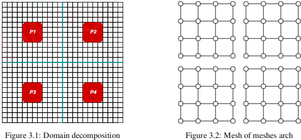
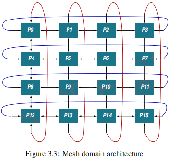
It is proposed to modify the domain decomposition by a parallel mesh-of-meshes architec- ture style as shown in Figure 3.2 for a 2 × 2 domain decomposition. Every grid point of each domain will contain an embedded virtual processor, however, only the top left corner domain, Domain(0y 0), will contain a corresponding mesh of physical processors. The computational model is simple. The processor mesh computes in parallel Domain(0y 0) then it switches onto Domain(0y 1), Domain(0y 2) and so on, sweeping through the domains horizontally and vertically, step by step, until it reaches the bottom right corner domain.
In general, let N × N be the original grid matrix which is partitioned into Q × Q domains such that every domain has M × M grid nodes where N = M × Q. Thus every full iteration through the entire grid consists of Q2 iterations through each of the Q2 domains.
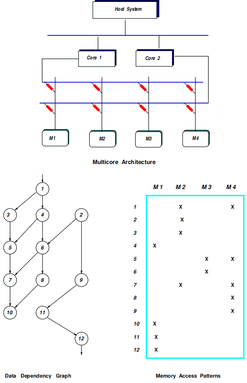
To achieves this, every physical processor node should have sufficient local storage to hold the intermediate results of corresponding nodes when going from domain to domain. However, to allow for inter communications between near neighboring domain nodes, we will use a wrap around or torus structure for the physical processor mesh shown in Fig. 3.3.
In what follows we assume that we will use the above Q × Q architecture Figs 3.2, 3.3 to solve the Poisson potential equation on a N ×N grid. The context switching time from domain to domain may be few cycles, say 5 (instruction) cycles. The grid has been initialized and the initials of every
node are stored in the corresponding processors. Specifically, the initial potential value of the top grid nodes is 100 whereas all others are initialized to zero.
3.2 Estimate the computation time for your solution assuming that the problem converges after 1000 iterations.
3.3 Estimate the speedup of the proposed approach (if any) in comparison to the standard domain decomposition technique in Figure 3.1. To be fair you should use the same number of processors Q2 and same grid size N × N for the domain decomposition in Figure 3.1.
3.4 You should write a C/C++ model for your Poisson solver and simulate your solution to find the convergence values of all nodes in the mesh assuming that the top boundary initial values do not change. Assume that N = 104 and Q = 103 .
3.5 Get some additional results for different grid sizes N × N. However, only a fraction of your results will be needed in your answers.
Problem 4. – Consider a 5-dimensional hypercube system, Hyper-5. Assume that you are to calculate all partial sums of the i items up to the sum of 32 items.
4.1 Construct a program for Hyper-5 that performs this operation in a time that grows as O(logN) if the number of processors is N. Assume that every processor node in the computer executes the same program, although the program can be slightly different from node to node since the processors in the Hyper-5 are independent.
4.2 Show explicitly the instructions that send and receive data between processors. Invent instructions as you need them and describe what the instructions do. Include some type of instructions for synchronization that forces a processor to be idle until a neighboring processor sends a message sends a message or datum that enables computation to continue.
4.3 Which communication steps if any in your answers require communications with pro- cessors that are not among the five processors directly connected to a given processor? How do you propose to implement such communication in software (assume that the hardware itself does not provide remote communication as a basic instruction) ?
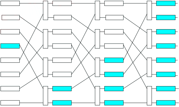
Problem 5. Consider a homogeneous multicore machine containing two single-thread processor cores and four shared memory modules, M1 y M2 y M3 y M4. The cores and memories are connected via a 2 × 4 cross bar switch. A program to be executed on the multicore system is represented by the data dependency graph of the following figure involving the instructions I1 y I2 y ●●●y I12. We assume instruction execution time 1 cycle, cross bar time 2 cycles and memory reference time 2 cycles. We also assume that the instruction execution and memory reference is consolidated or not pipelined. The memory access requirements for each instruction are given in the table. We do consider memory conflicts and cross bar conflicts.
There is a host processor which holds initially the instruction program. The host is responsible for loading this program on the multicore system. Based on the data dependencies, the host will load instruction parts to each core for parallel execution. Because of this loading, the cores do not go through the instruction fetch phase. Assume the decoding time is subsumed by the loading. Then for every instruction, each core needs to access the memory through the crossbar, follow the
access patterns, and get the data back to the core again through the crossbar. At the end of the computation, the results are in the registers of each core.
5.1 Make a suitable allocation mapping of instructions into the processors of the multicore system which requires as short as possible computation time.
5.2 Design an algorithm that will systematically solve this problem in this environment, i.e the 2-processor, 2 × 4 cross bar and 4-memory homogeneous multicore system, assuming acyclic program dependency graph.
5.3 Suppose that the single threaded 2-core system is replaced by 2-threaded single processor core, keeping the four memory modules and replacing the cross bar by a bus. However, the instruction execution time is now 2 cycles, the bus transport time averages 1 cycle and the memory reference time remains 2 cycles. Consider that the data flow program graph consists of two program threads, i.e.
T1 : I1 y I3 y I4 y I5 y I6 y I7 y I8 y I10 and T2 : I2 y I9 y I11 y I12
Redo the above mapping problem 5.1 for the 2-threaded single core system assuming an additional 1 cycle context-switching penalty. Compare the results to the single threaded 2-core system, problem 5.1.
Problem 6. – A multiprocessor node must sometimes send a message to more than one other
processor, a task referred to as ”broadcasting”. Suppose that a node P0 in an n-dimensional hyper- cube system has to broadcast a message to all 2n _ 1 other processors. The broadcasting is subject to the constraints that the message can be forwarded (retransmitted) by a node only to a neigh- boring node, and each node can transmit only one message at a time. Assume that each message transmission between adjacent nodes requires only one time unit. In a two-dimensional system, for example, P0 could broadcast a message MESS as follows. At time t = 0, P0 sends MESS to P1 . At t = 1, P0 sends MESS to P2 and P1 sends MESS to P3, thus completing the broadcast in 2 time units.
6.1 Construct a general broadcasting algorithm for the n-dimensional case that allows a mes- sage to reach all nodes in n time units. Specify clearly the algorithm used by each node to determine the neighboring nodes to which it should forward an incoming message.
6.2 Apply your algorithm on the designing the 8 × 8 heat-flow program (Laplace equation) to run on a 64-processor hypercube computer that simulates a mesh computer. Specify com- pletely the function you use to map the problem’s gridpoints onto the nodes of the hypercube.
6.3 Simulate the 16 × 16 heat-flow problem, i.e. build a C/C++ program to simulate the op- eration of a net of 2 × 2 processor nodes, assuming reasonable communication cost. Tabulate your results. Comment how would the problem scale to a 256 × 256 heat-flow problem?
Problem 7. – Consider the following arithmetic expression:
F = (A0 + A1 + ... + A7) × (B0 + B1 + ... + B7)
7.1 Show a minimal height tree implementation of F assuming unlimited processors. Com- pute the speedup S1 and the efficiency E1 .
7.2 Find a minimal height tree implementation of F assuming 4 (four) processors available each being able to execute the addition or multiplication operation in one time step. Compute the speedup and efficiency, S2 and E2, respectively.
7.3 Suppose you want to implement F using a 4 × 4 mesh connected network. a) Describe a procedure that implements F in minimal time on the mesh network, also find the speedup and efficiency of your parallel mesh implementation. b) If your boundary processors are connected by end-around or wrap-around connections (toroidal connections), show how your solution improves in terms of the speedup and efficiency.
7.4 Suppose you want to implement F using 8 (eight) processors connected into a 8 node shuffle network using 4 switching elements and feedback paths (similar network shown in class). Describe an algorithm that implements F in minimal time using this shuffle network. Assume that the switches can shuffle a data set in one time step, during the same time the processors perform an operation on another data set. Compute the speedup and efficiency, S3 and E3, respectively.
7.5 Suppose that we want to implement F using a 4-dimensional hypercube network. As- sume that the 16 variables Ai and Bi , i= 0,1,...,7 have already been loaded to the 16 nodes of the cube. Describe an algorithm that will implement F in minimal time using this hypercube network. Compute S4 and E4 .
7.6 Discuss the pros and cons of the above 5 implementations.
Problem 8. – The purpose of this problem is to explore some of the properties of the perfect shuffle scheme.
8.1 Consider a processor that has the perfect shuffle and pair-wise exchange connections shown in Figure bellow. For an eight-processor system, show that the permutation that cyclically shifts the input vector by three positions is realized by some setting of the ex- change modules. Draw the network unrolled in time to show the setting that realizes this permutation.
8.2 Repeat the above problem question to show that a cyclical shift of two positions is real- izable.
8.3 Prove a shuffle-exchange network can realize any cyclical shift in log2N iterations for an N-processor system when N is a power of 2.
Perfect shuffle network. Tall boxes depict modules that can exchage their inputs.
Shaded modules are reachedfrom Processor 3 via some sequence of shuffle−exchange
![]()
Problem 9. – Consider the use of a four-PE array processor (PE means processing element or processor) to multiply two 3 × 3 matrices. The interconnection structure of the four PEs is shown in Figure below. Wraparound connections appear in all rows and columns of the array. You need to map the matrix elements initially one onto each of the processors. All the three multiplications needed for each output element cij must be performed in the same PE in order to accumulate the sum of products. Of course, you are allowed to shift the matrix elements around if needed.
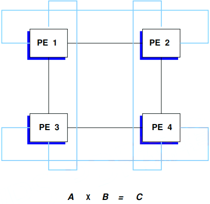
9.3 Parallel shifts are carried out in the horizontal and vertical directions. Show the mapping of the A and B matrix elements before the second group of multiplications can be carried out.
9.4 What are the multiplications to be carried out in each processor without any further shifting? (Don’t bother with summing with the previous terms. Summation operations in dot product operations are embeded in the multiply hardware automatically.)
9.5 Suppose the two matrices have already been allocated as in problem part 9.1. Assume each processor can perform one multiplication per unit time or one shift in a single direction per unit time for each number. (If you shift two numbers, it takes two units of time.) Deter- mine the time units needed to complete parts 9.1, 9.2, 9.3, 9.4, respectively. Minimizing the total time delay is the design goal.
Problem 10. – In this problem you will implement the 3D heat transfer equation on a cubical solid volume N × N × N. You should develop your solution code in C++ using the OpenMP Library. Your code should be multi-threaded to run in parallel on any modern multicore system, desktop or laptop. You will need to install the opensource tools gcc, g++ and the OpenMP Library. This installation task should be fairly easy to do on any recent Linux distribution, or on a virtual Linux on top of the Windows platform.
To help you with your parallel programming task, we provide a parallel C++ code, which is
well documented, and is also attached in the file: 1Dheat-omp.cpp
This code solves the heat transfer problem on a 1-dimensional wire.
To compile this program just do:
g++ -fopenmp 1Dheat transfer.cpp -o 1Dheat transfer
10.1 Read the attached program and its comments carefully to understand how it works, especially the code’s parallel sections. Modify and expand the 1D code to produce a parallel heat transfer solver for the 3D cubical volume.
10.2 Generate some example cases and results by varying the problem parameters such as the threshold, initializations, boundary heat conditions, and the volume size.
10.3 For performance comparison you should generate a serial solution program which im- plements the same 3D volume running on a single core processor. Compare the multicore to the single processor speedup over several example cases. What happens if the volume size is not large enough?
Note: when running, the parallel program will produce as many threads as the number of mul- ticores in your desktop, one thread for each core. You can change this behavior by setting the environment variable OMP NUM THREADS to the number of threads desired, however, your perfor- mance may vary. You can also do this within the C++ code itself.
2021-12-07