Hello, dear friend, you can consult us at any time if you have any questions, add WeChat: daixieit

ISGB-799V Homework #4: Probability Distributions

The Geometric Probability Distribution & Weak Law of Large Numbers

A random variable with the geometric probability distribution is associated with an experiment that shares some of the characteristics of a binomial experiment. This experiment also involves identical and independent

trials, each of which can result in one of two outcomes: success or failure. The probability of success is equal to p and is constant from trial to trial. However, instead of the number of successes that occur in n trials, the geometric random variable is the number of trials on which the first success occurs. The geometric probability distribution is often used to model distributions of lengths of waiting times.

Let us roll a K sided die with numbers 1, .  .  .  , K written on them where K > 1. Each number is equally likely to be rolled. Let X be a random variable representing the number of rolls needed to get the number K for the first time.  (Note: number of rolls includes the roll where K appears.)

1.  On any roll, what is the probability of rolling the value K?

2. What are all of the possible values of X ?

3.  Create a function with arguments, K and simulations, with simulations representing the number of times we should play out this scenario. Your function should return the number of times the die was rolled in order to get the value K. (Helpful hint: Try using a while loop)

4.  For K = [2, 6, 12, 15] simulate 100 rounds of the scenario and plot each set of results with a bar graph.

5.  Repeat question 4 by simulating 100 new rounds of each scenario and plot the results. Have your results changed? Please explain how they have changed. Why might your results be different?

6.  For each combination of ‘ simulations = [100, 1000, 5000, 20000] and K = [2, 6, 12, 15] calculate the average number of rolls required to get K. Show these results in a table where your columns are values of n_sim and your rows are values of K .

7.  How would you describe a general formula for calculating the average number of rolls?

8.  For K = 6 and simulations = 1000, estimate the following probabilities using your simulation function:

10.  Given that the probability mass function for the a geometric distributed random variable X is9. In theory, is the probability P (X = 500) > 0 when K = 6? Explain.

Use the functions dgeom() and pgeom() to calculate the probabilites in question 8. For the x arguments, enter the outcomes x-1 and your answer for #1 for the argument prob.  (Hint: Check ?dgeom if you need help)

11.  Create a figure with two plots side by side: The first plot of the empirical probability mass function estimate based on the data simulated in #8 (histogram is acceptable - use prob=TRUE). The second plot should plot the theorical probability mass function for our data in #10.

12.  How close are your answers from your simulation to the probabilities from the geometric distribution you just created? Describe this given what we’ve learned about the Weak Law of Large Numbers in lecture 8. What parameters need to change in our function in order for our empirical probabilities to match the theoretical values for (X = x)

13.  For K = 6, and simulations = [1 - 5000] (Hint: use a for loop) plot the mean of each sample as a line graph. Add a horizontal line at the theorical mean (6). What is your observation of this relationship between n_sim and the mean of our sample? If your code takes longer than 5 minutes to run you may reduce the simulations to a lower number.

14.  For K = 6, what is the probability that it takes more than 12 rolls to roll a 6?

15.  For K = 6, what is the probability that you roll a 6 in your first three rolls?

16.  For K = 6, what is the 95th percentile for number of rolls required to roll a 6?

The Exponential Probability Distribution & Central Limit Theorem

The magnitude of earthquakes in North America can be modeled as having an exponential distribution with mean µ of 2.4.

For an exponential distribution :

Mean: E [X] = λ

Variance: E [X2] − (E [X])2  = λ2

18.  Simulate 1000 earthquakes and plot the distribution of Richter Scale values (Hint:  rexp(x,  rate =  1/lambda)).  Let this data represent X.  Create a histogram of X and describe the shape of this distribution. How does this differ from the normal distribution?

19.  Find the probability that an earthquake occurring in North America will fall between 2 and 4 on the Richter Scale.

20.  How rare is an earthquake with a Richter Scale value of greater than 9?

21.  Create a function which will simulate multiple samples drawn from an exponential distribution with λ = 2.4 (Hint: rexp(x,  rate  =  1/lambda) and return a vector containing the mean values for each of your samples. Your arguments should be lamba, simulations for the number of simulations per sample, and n (sample size) for the number of samples of size simulations to be created.

22.  Use your function with arguments lambda = 2.4, simulations = 1000, n = 40 to create a vector of sample mean values of Richter Scale readings. Let  represent this data. Plot a histogram of the data. Describe the distribution of . Is  distributed differently than X ?

23.  Calculate the sample mean and sample variance for the data simulated in #18. Calculate the population variance given λ = 2.4.

24.  Create a plot of . Make sure to set prob=TRUE in the hist() function. Include vertical lines for the sample and theoretical mean values (red = sample mean, blue = theoretical mean).

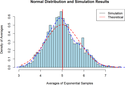
25.  Add lines to our plot of  to plot the density for both our simulated sample and theoretical population (Hint: use dnorm(x, mean=lambda,  sd=(lambda/sqrt(n)) to calculate theorical population density). Make sure to set prob=TRUE in the hist() function. See the example plot below for guidance:

26.  The Central Limit Theorem states that if you take many repeated samples from a population, and calculate the averages or sum of each one, the collection of those averages will be normally distributed. Does the shape of the distribution of X matter with respect to the distribution of ? Is this true for all any parent distribution of ?

27. What will happen to the distribution of  if you re-run your function with arguments lambda = 2.4, simulations = 10000, n = 40?  How does the variance of  change from our data simulated for  in #25?  Create a figure with the histograms (prob=TRUE) for both of our  sampling distributions. Explain the difference in the two distributions of  (simulations = 1000, simulations = 10000).

28.  Now explore what will happen to the distribution of  if you re-run your function with arguments lambda = 2.4, simulations = 10000, n = 10? How does the variance of  change from our data simulated for  in #25? Create a figure with the histograms (prob=TRUE) for our  sampling distributions (n = 40, n = 10). Explain the difference in the two distributions of 

29. In 3-4 sentences, summarize your findings for questions 26-28. What role does n (sample size) play in the variance of ?

EXTRA CREDIT: Choose a probability distribution that we have not studied in class and repeat the above exercises.