COMP5930M - Scientific Computing

Coursework 2

Task

The numbered sections of this document describe problems which are modelled by partial differ- ential equations. A numerical model is specified which leads to a nonlinear system of equations. You will use one or more of the algorithms we have covered in the module to produce a numerical solution.

Matlab scripts referred to in this document can be downloaded from Minerva under Learning Resources / Coursework.  Matlab implementations of some algorithms have been provided as part of the module but you can implement your solutions in any other language if you prefer.

You should submit your answers as a single PDF document via Minerva before the stated deadline. MATLAB code submitted as part of your answers should be included in the document. MATLAB functions should include appropriate help information that describe the purpose and use of that function.

Standard late penalties apply for work submitted after the deadline.

Disclaimer

This is intended as an individual piece of work and, while discussion of the work is encouraged, plagiarism of writing or code in any form is strictly prohibited.

1.  A one-dimensional PDE: Nonlinear parabolic equation

[20 marks total]

Consider the nonlinear parabolic PDE: find u(x, t) such that

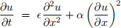
in the spatial interval x e (0, 1) and time domain t > 0.

Here c and α are known, positive, constants.

Boundary conditions are specified as u(0) = 0 and u(1) = 1.

Initial conditions are specified at t = 0 as u(x, 0) = x.

We numerically approximate (1) using the method of lines on a uniform spatial grid with

m nodes on the interval [0, 1] with grid spacing h, and a fixed time step of ∆t.     Code for this problem can be downloaded from Minerva and is in the Q1/ folder.

(a) Find the fully discrete formulation for (1) using the ce。tr。h f。Nte dN度ere。ce fpr。uh。s

Define the nonlinear system F(U) = 0 that needs to be solved at each time step to obtain a numerical solution of the PDE (1).

(b)  Solve the problem for different problem sizes:  N = 81, 161, 321, 641 (choose m ap- propriately for each case).  Use NT  = 40 time steps.  Create a table that shows the total computational time taken T, the total number of Newton iterations S, and the average number of Newton iterations per time step TS  = T/S.  Time the execution of your code using Matlab functions tic and toc. Show for each different N :

i. the total number of unknowns, N

ii. the total computational time taken, T

iii. the total number of Newton iterations, S

iv. the average time spent per Newton iteration, tS  = T/S

Estimate the algorithmic cost of one Newton iteration as a function of the number of equations N from this simulation data. Does your observation match the theoretical cost of the algorithms you have used?

Hint: Take the values N and the measured tS (N) and fit a curve of the form tS  = CNP  by taking logarithms in both sides of the equation to arrive at

log tS  = log C + P log N,

then use polyfit(  log(N),  log(tS),  1  ) to find the P that best fits your data. (c)  Derive the exact expression for row i of the Jacobian for this problem.

How many nonzero elements are on each row of the Jacobian matrix?

(d)  Repeat the timing experiment (c), but using now the Thomas algorithm sparseThomas.m to solve the linear system and the tridiagonal implementation of the numerical Ja-     cobian computation tridiagonalJacobian.m.  You will need to modify the code to

call newtonAlgorithm.m appropriately.

Create a table that shows for each different N :

i. the total number of unknowns, N

ii. the total computational time taken, T

iii. the total number of Newton iterations, S

iv. the average time spent per Newton iteration, tS  = T/S

Estimate the algorithmic cost of one Newton iteration as a function of the number of equations N from this set of simulations. Does your observation match the theoretical cost of the algorithms you have used?

Hint: Take the values N and the measured tS (N) and fit a curve of the form

tS  = CNP  by taking logarithms in both sides of the equation to arrive at

log tS  = log C + P log N,

then use polyfit(  log(N),  log(tS),  1  ) to find the P that best fits your data.

2.  A three-dimensional PDE: Nonlinear diffusion

[20 marks total]

Consider the following PDE for u(x, y, z):

defined on [x, y, z] e [一10, 10]3  with u(x, y, z) = 0 on the boundary of the domain, and some known function g(x, y, z) that does not depend on u.

Using a finite difference approximation to the PDE (2) on a uniform grid, with grid size h and n nodes in each coordinate direction, the nonlinear equation Fijk  = 0 to be solved at an internal node may be written as

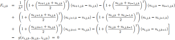
Code for this problem can be downloaded from Minerva and is in the Q2/ folder.  The Matlab function  runFDM.m controls the numerical simulation of the discrete nonlinear system (3).

(a)  Run the model using runFDM.m with grid dimension m = 5, 8 and 11 for tol = 10 −8 and initial guess u(x, 0) = 0 for all x. Create a table that shows for each different N :

i. the total number of unknowns, N

ii. the total computational time taken, T

iii. the total number of Newton iterations, S

iv. the average time spent per Newton iteration, tS  = T/S

Estimate the algorithmic cost of a single Newton iteration in terms of the size of the nonlinear system N , i.e.  T  =  b(Np ).  How does it compare to the theoretical worst-case complexity?

Hint:  Take the values N and the measured tS (N) and fit a curve of the form tS  = CNP  by taking logarithms in both sides of the equation to arrive at

log tS  = log C + P log N,

then use polyfit(  log(N),  log(tS),  1  ) to find the P that best fits your data.

(b)  Replace in runFDM.m the call to a dense Jacobian implementation fnJacobian.m with

a call to a sparse implementation, buildJacobian.m.  You will need to uncomment the following function calls before calling the Newton algorithm:

[  A,  nz  ]  =  sparsePattern3DFD( m  );  %  3d  FDM  sparsity  pattern

[  loc,  nf  ]  =  sparseJac(  A,N  );         %  function  calls  required  to  evaluate  J

i. Visualise the sparsity pattern of A using the command spy in the case m = 8 and include the plot in your report.  Note:  The matrix A has the same sparsity pattern as the Jacobian for this problem.

ii. Use the command lu to compute the LU-factorisation of A in the case m = 8. What are the number of non-zero elements L and U , respectively?

iii. Visualise the sparsity pattern of the LU-factors using the command  spy and include the plot in your report.  Can you observe something unexpected about the matrix L? How can you explain this perceived discrepancy?

iv. Use these matrices as an example to explain what we mean by fhh)N。 of the LU-factors.

(c) Use the MATLAB code provided to assemble the Jacobian matrix J for problem (2) with the grid size m = 8, and consider solving the linear problem Jx = b, where b = [1, 1, 1, . . . , 1]T . Solve this linear problem using three different solution methods:

i. LU-decomposition direct method (directLU.m);

ii.  Jacobi iterative method (jacobi.m) using the initial guess x0 = b and tol = 10 −6 ;

iii.  Gauss-Seidel iterative method (gaussseidel.m) using the initial guess x0  = b and tol = 10 −6 .

Solve the problem 100 times with each method and report the total time used for each method (hint: use the commands tic and toc), plus for the iterative methods the number of iterations taken.

(d)  Replace in runFDM.m the call to linearSolve.m function that uses dense linear alge- bra with the alternative matlabLinearSolve.m that uses sparse linear algebra. Solve the problem using the sparse implementation for m = 15, 19 and 23. Create a table that shows for each different N :

i. the total number of unknowns, N

ii. the total computational time taken, T

iii. the total number of Newton iterations, S

iv. the average time spent per Newton iteration, tS  = T/S

Estimate the algorithmic cost of this new sparsity-based implementation using the timings of the numerical experiments. Compare the results with those of 2(a).          Hint:  Take the values N and the measured tS (N) and fit a curve of the form tS  = CNP  by taking logarithms in both sides of the equation to arrive at

log tS  = log C + P log N,

then use polyfit(  log(N),  log(tS),  1  ) to find the P that best fits your data.