Hello, dear friend, you can consult us at any time if you have any questions, add WeChat: daixieit

Homework #4

FE-570 Fall 2021

Glosten-Harris  model.  In Lecture 8 we learned about the Glosten- Harris model.  This is an improved version of the Roll model which takes into account:

。  Bid-ask bounce cdt

。  Price impact λzt

In this model the trade price 夕t  is given by

(1)                                        夕t  = mt + cdt + λzt

where the efficient price mt  contains also a price impact λzt − l  due to the previous trade

(2)                                     mt  = mt − l + λzt − l + ut

Here ut  are iid random variables with mean zero and variance σu(2), just like in

the Roll model.

Note that here zt  are signed trade sizes:  positive for buy, negative for sell.

Calibrate the λ．c parameters of this model on the JPM tick level dataset in taqdata JPM 20210113 ESTMktHrs.RData.

For this analysis it is important to use only trades executed on one ex- change, as different exchanges have different price impact. For this problem use only the trades executed on ADF. Also exclude from the analysis large trades at the start and end of the trading session.  For example keep only trades with time stamps between 10:00am - 12:00pm.

Use getTradeDirection to estimate the trade signs dt .

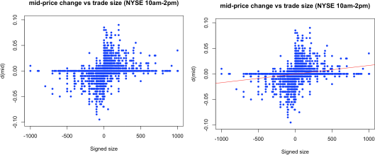
Figure 1: Mid-price change vs (signed) trade size |zt |dt . Sample results, using EX==NYS and time stamps 10:00am-2:00pm.

Hints

First, we need the signed trade sizes zt  = dt |zt |, where dt  are the trade indicators and |zt | are the absolute values of the trade size which are available in the TAQ data as tqdata$SIZE. We get the trade indicators using the getTradeDirection(tqdata) which is the implementation of the Lee-Ready mid-point criterion.

The calibration proceeds in two steps.

Step 1. Determine λ. This is done using Equation (2) where we assume that the efficient price mt  is the same as the mid-price  (αt +ót ). The change of the efficient price from one trade to the next is

(3)                               ∆mt  = mt · mt − l  = λzt − l + ut

A linear regression of ∆m with respect to z(t · 1) of the form ∆m = αz(t · 1) + ó should give λ as the slope, and ó = E[ui] the average of the residuals.

Sample numerical results are shown in Figure 1, using trades executed on NYSE between 10:00am-2:00pm. The regression is shown as the red line in the right plot of Figure 1.  The parameter λ has an interpretation as a measure of price impact. The price impact is positive for a buy, and negative for a sell.

Step 2. Determine c. This is done from Eq. (1) written as

(4)                                        夕t · mt · λzt  = cdt

A linear fit of the left-hand side to the dt  should give c as the slope.