MATH GR 5280, Capital Markets & Investments
Hello, dear friend, you can consult us at any time if you have any questions, add WeChat: daixieit
![]() MATH GR 5280, Capital Markets & Investments
MATH GR 5280, Capital Markets & Investments
Final Project
Note: All files and information related to the final project are located in the folder “Final Project”.
The aim of this Final Project is to practically implement the ideas from the course, specifically from Chapters 7 and 8. You will be given a recent 20 years of historical daily total return data for ten stocks, which belong in groups to three-four different sectors (according to Yahoo!finance), one (S&P 500) equity index (a total of eleven risky assets) and a proxy for risk-free rate (1-month Fed Funds rate). In order to reduce the non-Gaussian effects, you will need to aggregate the daily data to the monthly observations, and based on those monthly observations, you will need to calculate all proper optimization inputs for the full Markowitz Model (“MM”), alongside the Index Model (“IM”). Using these optimization inputs for MM and IM you will need to find the regions of permissible portfolios (efficient frontier, minimal risk portfolio, optimal portfolio, and minimal return portfolios frontier) for the following five cases of the additional constraints:
1. This additional optimization constraint is designed to simulate the Regulation T by FINRA (https://www.finra.org/rules-guidance/key-topics/margin-accounts), which allows broker-dealers to allow their customers to have positions, 50% or more of which are funded by the customer’s account equity:
![]()
![]() wi
wi![]() ≤ 2 ; i =1
≤ 2 ; i =1
Note that this is a difficult-to-converge case which requires “regularization” discussed in the
class, that is replace ![]() wi
wi![]() in the above constraint with
in the above constraint with ![]() , where δ= 0.001 .
, where δ= 0.001 .
2. This additional optimization constraint is designed to simulate some arbitrary “box” constraints on weights, which may be provided by the client:
![]() wi
wi ![]() ≤ 1, for ∀i ;
≤ 1, for ∀i ;
3. A “free” problem, without any additional optimization constraints, to illustrate how the area of permissible portfolios in general and the efficient frontier in particular look like if you have no constraints;
4. This additional optimization constraint is designed to simulate the typical limitations existing in the U.S. mutual fund industry: a U.S. open-ended mutual fund is not allowed to have any short positions, for details see the Investment Company Act of 1940, Section 12(a)(3)
(https://www.law.cornell.edu/uscode/text/15/80a-12):
wi ≥ 0, for ∀i ;
5. Lastly, we would like to see if the inclusion of the broad index into our portfolio has positive or
negative effect, for that we would like to consider an additional optimization constraint: w1 = 0 .
You will need to present the results in both the tabular and graphical form with the objective to make inferences and comparisons between the sets of constraints for each optimization problem and between the MM and IM models in general. The grading will be done by comparing your tabulated results to exact solutions.
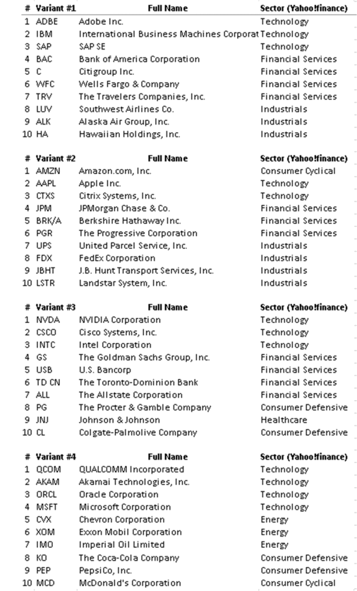
Again, you will be given 20 years of daily data of total returns for the S&P 500 index (ticker symbol “SPX”), and for ten stocks (ticker symbols see the table below) such that there are three-four groups of stocks with stocks in each group belonging to one (Yahoo!finance) sector and an instrument representing risk-free rate, 1-month annual Fed Funds rate (ticker symbol “FEDL01”). Note that stocks in each variant
are completely different. Therefore, each groups will have its own results and conclusions.
Below, please, find the table of stock ticker symbols (aka, tickers) for each group to work with:
|
|
Variant #1 |
Variant #2 |
Variant #3 |
Variant #4 |
|
Index |
SPX |
SPX |
SPX |
SPX |
|
Stock #1 |
ADBE |
AMZN |
NVDA |
QCOM |
|
Stock #2 |
IBM |
AAPL |
CSCO |
AKAM |
|
Stock #3 |
SAP |
CTXS |
INTC |
ORCL |
|
Stock #4 |
BAC |
JPM |
GS |
MSFT |
|
Stock #5 |
C |
BRK/A |
USB |
CVX |
|
Stock #6 |
WFC |
PGR |
TD CN |
XOM |
|
Stock #7 |
TRV |
UPS |
ALL |
IMO |
|
Stock #8 |
LUK |
FDX |
PG |
KO |
|
Stock #9 |
ALK |
JBHT |
JNJ |
PEP |
|
Stock #10 |
HA |
LSTR |
CL |
MCD |
|
Risk-free rate |
FEDL01 |
FEDL01 |
FEDL01 |
FEDL01 |
Below, please, find the table which shows the details for each of the stocks and which stocks belong to the same sector in each variant.
Using this data you will need to prepare an Excel spreadsheet that makes all the necessary calculations to plot a Permissible Portfolios Region, which combines the Efficient Frontier, the Minimal Risk or Variance Frontier, and the Minimal Return Frontier for a given set of constraints (1-5 above). The Minimal Return
Frontier and the Efficient Frontier together are forming the Minimal Risk or Variance Frontier – it is just a matter of re-formulating the optimization problem, as follows:
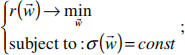
Minimal Return Frontier:
Two unique points that you need to find on the Efficient Frontier are of special interest:
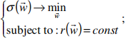
Minimal Risk Portfolio:

and
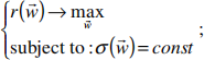
Efficient Risky Portfolio:
This Final Project in an open-book which means that you can and should use the Instructor’s handouts and the corresponding Chapter copy reading material provided by the Instructor, as well as any additional materials provided to you. Instructor and TAs have performed all these calculations for each of the variant’s portfolios and will be able to compare your numbers, specific points and graphs to theirs. If your spreadsheet calculations are done correctly, you and we should be able to match the results with sufficient accuracy.
The main tool that we would like you to use to solve the optimization problems for each point on the Minimal Risk or Variance Frontier is the Excel Solver. Please, try to learn how to use it on your own, if you have not done so already. The TAs will be helping you to address any issues related to Solver during their office hours. To calculate large numbers of multiple points on any of the required frontiers, you will need to use the Excel Solver Table, which the TAs will teach you how to install and use. Both Excel Solver and Excel Solver Table will also be covered in lectures with illustrations which are very similar to your Final Project.
For your calculations, you need to use the full available historical data range:
• start date 5/11/2001;
• end date 5/12/2021.
As it was mentioned above, you will need to calculate the solutions to two optimizations covered in lectures:
• The full Markowitz Model (MM);
• The Index Model (IM).
As we have described this in detail above, each of these optimization problems MM and IM you will need to implements and solve with the following additional optimization constraints:
1. ![]()
![]() wi
wi ![]() ≤ 2 ; i=1
≤ 2 ; i=1
2. ![]() wi
wi ![]() ≤ 1, for ∀i ;
≤ 1, for ∀i ;
3. no constraints;
4. wi ≥ 0, for ∀i ;
5. w1 = 0 .
As we have already mentioned, your task is to produce the following objects on the Permissible Portfolios Region in the graphical form:
1. Minimal Risk or Variance Frontier (a curve), range for portfolio returns: from -10% to 50% with step of 0.5%;
2. Global Minimal Risk or Variance Portfolio (a point);
3. Maximal Sharpe Ratio or Efficient Risky Portfolio (a point);
4. Maximal Return or Efficient Frontier (a curve), range for portfolio standard deviation: from 10% to 50% with step of 0.5%;
5. Capital Allocation Line or CAL (a straight line);
6. Minimal Return or Inefficient Frontier (a curve), range for portfolio standard deviation: from 10% to 50% with step of 0.5%.
The curves above must be also produced in tabular form (Excel), with which comparison for grading will be made, using specifically the above ranges. If a numerical solution cannot be found, just leave the corresponding cell empty. The points above should also be tabulated. All the tabulation should be done similar to example provided by the Instructor (see the file “Final Project Variant0.xlsx” provided).
As a single value for the risk-free rate to draw the CAL, please, use the very last value of the “FEDL01” time series.
You should analyze all your results with the purpose of comparison of different constraints for each optimization problem (MM and IM), and the two optimization problem solutions between each other with same constraints.
Do not hesitate to ask Lecturer or TAs any questions related to this.
Good luck!
You are given two weeks to complete the Final Project and to prepare the presentations. We encourage you not to delay starting the work as workload is meant for several days of team work and not as a one- night, single person effort.
Final Project is due as an Excel file with the graphs and tables requested, on December 11th, 2021 at 7:00 AM EST.
2021-12-03