Hello, dear friend, you can consult us at any time if you have any questions, add WeChat: daixieit

Quantitative Methods 1

Problem Set 4: Regression Discontinuity

1. Consider the following regression output and scatter plot

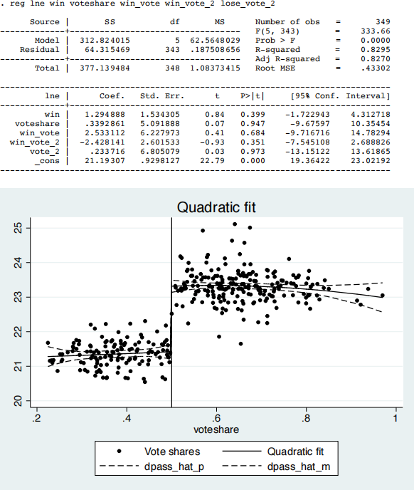
where lne is ln expenditure at the district level, voteshare is the Democratic vote share  (0 to 1), win is an indicator for voteshare > 0.5, win_vote is win x vote, vote_2 is voteshare x voteshare, and win_vote_2 is win x vote x vote. What is the exact value of the jump at 0.5? Express this it as the appropriate combination ofregression coefficients from the results table above.

The data for questions 2-7 are taken from Damon Clark “Politics, Markets and           Schools: Quasi-Experimental Evidence on the Impact ofAutonomy and Competition from a Truly Revolutionary UK Reform”.

This can be downloaded our web directory.

The basic idea of the paper can be described very simply.

Traditionally schools in the UK have been funded and managed by Local Education Authorities (in London, this would be a borough e.g. Camden, Westminster) with     rather little in the way of autonomy given to individual schools.  But the 1988           Education Act allowed schools to opt out ofLEA control and become funded by      central not local government with much more autonomy – this was called ‘grant-      maintained’.  Schools could become GM if a simple majority of parents chose that   option in a ballot.  So if 51% of parents voted for GM status that school would          become a GM-school while if49% voted for it, it would remain under LEA control. This is the basis of the regression discontinuity design.

The paper can be thought of as contributing more generally to the debate about how    public institutions like schools or hospitals should be run – should they be given a       budget and left to spend it how they want or should they be more tightly controlled.     In the case of GM schools, becoming GM resulted not just in more autonomy but also more resources which were justified as the school now had to deal with some issues    that had previously been handled by the LEA but which some people felt were bribes  as the government wanted to encourage the growth of GM schools.  So the change to  GM resulted in both more autonomy and possibly more resources.

The data set consists of a small number ofvariables:

-    passrate0 : the pass rate of pupils in the school in the year immediately prior to the vote

-     passrate2 : the pass rate of pupils in the school two years after the vote

-     dpass: the change in the pass rate = passrate2-passrate0

-     vote: the percentage vote in favour ofthe GM status

-     win: a dummy variable ifthe vote was more than 50%

2.          Do a scatter-plot ofthe change in the pass rate on the vote in favour of GM     status.  Then superimpose a quadratic fit of a regression of dpass on vote, where you   allow the relationship to jump at the threshold; also include the +/- 2 standard errors   of the prediction. Now try the same with a cubic fit. Finally use a local polynomial fit (for the local polynomial you don’t need the standard error bands).

Bonus points (optional of course): Include the +/- two standard errors lines on the local polynomial fit.

3.         Reproduce the result in the first column of Table 3a of Clark

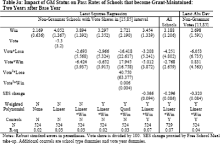
In this Table, Clark restricts his sample to those schools with votes in favour of GM  status between 15% and 85%.  Why did you think he chose this sample restriction?   Why do subsequent columns of Table 3a include functions ofthe vote share, both on their own and interacted with the win/lose variable?

Experiment with thresholds for sample inclusion that differ from the [15,85] chosen by Clark– how different are the results?  What are the trade-offs to be considered     here?  Why is the information in the scatter-plot useful in considering what               specification and sample to use?

4.         Instead of using dpass as the outcome variable, repeat your analyses using       passrate2 as the outcome variable.  What does the theory of regression discontinuity   say about the comparison ofthe results with this outcome variable compared to the     previous set of results?  How do they compare in practice?  Explain this. Now use the rd command to estimate the precise difference at the cutoff. How do you your results  differ?

5.         Someone critical of the results suggests using passrate0 as the dependent      variable.  They show that if one just regresses this on the win variable this has a       significant negative coefficient.  They argue this invalidates the regression                discontinuity design because winning should be uncorrelated with variables prior to the treatment.  Evaluate this argument using regressions and appropriate figures.

6.         Someone suggests that voteshares could have been manipulated. Use the   program DCdensity.ado from McCrary to test for this. You’ll find the program at

http://emlab.berkeley.edu/~jmccrary/DCdensity/,

where he also explains how to use it.

7. Explore sensitivity ofyour estimates to bandwidth choice. Begin with the optimal bandwidth, and then try a grid of bandwidths ranging from 75% to 125% ofthe         optimal bandwidth. Do you results seem sensitive or robust to bandwidth choice?     (Hint: install the stata program rd. Type help  rd. All of this is coded for you.)