COMP9334 Project, Term 1, 2024: Computing clusters
Hello, dear friend, you can consult us at any time if you have any questions, add WeChat: daixieit
COMP9334 Project, Term 1, 2024:
Computing clusters
Due Date: 5:00pm Friday 19 April 2024
Version 1.01
Change lo
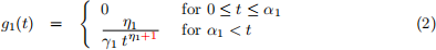
• Version 1.01 (27 March 2024). There is a mistake in the denominators of the two probability density functions in Section 5.1.1. For g0 (t), it should be t raised to the power of η0 +1 where the +1 was missing. A similar error appeared in g1 (t), it should be t raised to the power of η 1 +1.
• Version 1.00. Issued on 19 March 2024.
1 Introduction and learning objectives
You have learnt in Week 4A’s lecture that a high variability of inter-arrival times or service times can cause a high response time. Measurements from real computer clusters have found that the service times in these clusters have very high variability [1]. The reference paper [1] also has a number of suggestions to deal with this issue. One suggestion is to separate the jobs according to their service time requirements, and have one set of servers processing jobs with short service times and another set of servers for jobs with long service times. This arrangement is the same as supermarkets having express checkouts for customers buying not more than a certain number of items and other checkouts that do not have a limit on the number of items. You had seen this theory in action in Week 4A’s revision Problem 1. We also highly recommend you to read the paper [1].
In this project, you will use simulation to study how to reduce the response timef a server farm that uses different servers to process jobs with different service time requirements.
In this project, you will learn:
1. To use discrete event simulation to simulate a computer system
2. To use simulation to solve a design problem
3. To use statistically sound methods to analyse simulation outputs
We mentioned a number of times in the lectures that simulation is not simply about writing simulation programs. While it is important to get your simulation code correct, it is also important that you use statistically sound methods to analyse simulation outputs. There, roughly half of the marks of this project is allocated to the simulation program, and the other half to statistical analysis; see Section 7.2.

2 Support provided and computing resources
If you have problems doing this project, you can post your question on the course forum. We strongly encourage you to do this as asking questions and trying to answer them is a great way to learn. Do not be afraid that your question may appear to be silly, the other students may very well have the same question! Please note that if your forum post shows part of your solution or code, you must mark that forum post private.
Another way to get help is to attend a consultation (see the Timetable section of the course website for dates and times).
If you need computing resources to run your simulation program, you can do it on the VLAB remote computing facility provided by the School. Information on VLAB is available here: https: //taggi.cse.unsw.edu.au/Vlab/
3 Multi-server system configuration with job isolation
The configuration of the multi-server system that you will use in this project is shown in Figure 1. The system consists of a dispatcher and n servers where n ≥ 2. The n servers are parti- tioned into 2 disjoint groups, called Groups 0 and 1, with at least one server in each group. The number of servers in Groups 0 and 1 are, respectively, n0 and n1 where n0 , n1 ≥ 1 and n0 +n1 = n.
The servers in Group 0 are used to process short jobs which require a processing time of no more than a time limit of Tlimit. The servers in Group 1 do not impose any limit on service time.
The dispatcher has two queues: Queue 0 and Queue 1. The jobs in Queue i (where i = 0, 1) are destined for servers in Group i. Both queues have infinite queueing spaces.
When a user submits a job to this multi-server system, the user needs to indicate whether the job is intended for the servers in Group 0 or Group 1. The following general processing steps are common to all incoming jobs:
• If a job is intended for a server in Group i (where i = 0, 1) arrives at the dispatcher, the job will be sent to a server in Group i if one is available, otherwise the job will join Queue i.
• When a job departs from a server in Group i, the server will check whether there is a job at the head of Queue i. If yes, the job will be admitted to the available server for processing.
Recall that the servers in Group 0 have a service time limit. The intention is that the users make an estimate of the service time requirement of their submitted jobs. If a user thinks that their job should be able to complete within Tlimit , then they submit it to Group 0; otherwise, they should send it to the Group 1.
Unfortunately, the service time estimated by the users is not always correct. It is possible that a user sends a job which cannot be completed within the time limit to Group 0. We will now explain how the multi-server system will process such a job. Since the user has indicated that the job is destined for Group 0, the job will be processed according to the general processing steps explained earlier. This means the job will receive processing by a server in Group 0. After this job has been processed for a time of Tlimit , the server says that the service time limit is up and will kill the job. The server will send the job to the dispatcher and tell it that this is a killed job. The dispatcher will check whether a server in Group 1 is available. If yes, the job will be send to an available server; otherwise, it will join Queue 1 to wait for a server to become available. When a server in Group 1 is available to work on this job, it will process the job from the beginning, i.e., all the previous processing in a Group 0 server is lost.
If a job has completed its processing at a Group 0 server, which means its service time is less than or equal to Tlimit , then the job leaves the multi-server system permanently. Similarly, a job completed its processing at a Group 1 server will leave the system permanently.
We make the following assumptions on the multi-server system in Figure 1. First, it takes the dispatcher negligible time to classify a job and to send a job to an available server. Second, it takes a negligible time for a server to send a killed job to the dispatcher. Third, it takes a negligible time for a server to inform the dispatcher on its availability. As a consequence of these assumptions, it means that: (1) If a job arriving at the dispatcher is to be sent to an available server right away, then its arrival time at the dispatcher is the same as its arrival time at the chosen server; (2) The departure time of a job from the dispatcher is the same as its arrival time at the chosen server; and (3) The departure time of a killed job from a server is the same as its arrival time at the dispatcher. Ultimately, these assumptions imply that the response time of the system depends only on the queues and the servers.
We have now completed our description of the operation of the system in Figure 1. We will provide a number of numerical examples to further explain its operation in Section 4.
You will see from the numerical examples in Section 4 that the number of Group 0 servers n0 can be used to influence the mean response time. So, a design problem that you will consider in this project is to determine the value of n0 to minimise the mean response time.
Remark 1 Some elements in the above description are realistic but some are not. Typically, users are required to specify a walltime as a service time limit when they submit their jobs to a computing cluster. If a server has already spent the specified walltime on the job, then the server will kill the job. All these are realistic.
The re-circulation of a killed job is normally not done. A user will typically have to resubmit a new job if it has been killed. If a killed job is re-circulated, then it may be given a lower priority, rather than joining the main queue which is the case here.
Some programming technique (e.g., checkpointing) allows a killed job or crashed job to resur- rect from the last state saved rather than from the beginning. However, that may require a sizeable memory space.
In order to make this project more do-able, we have simplified many of the settings. For example, we do not use lower priority for the re-circulated killed jobs.
4 Examples
We will now present three examples to illustrate the operation of the system that you will simulate in this project. In all these examples, we assume that the system is initially empty.
4.1 Example 0: n = 3, n0 = 1, n1 = 2 and Tlimit = 3
In this example, we assume the there are n = 3 servers in the farm with 1 (= n0 ) server in Group
0 and 2 (= n1 ) servers in Group 1. The time limit for Group 0 processing is Tlimit = 3.
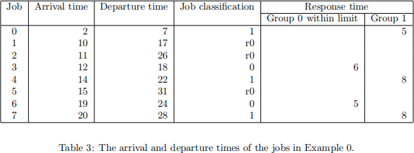
Table 1 shows the attributes of the 8 jobs that we will use in this example. Each job is given an index (from 0 to 7). For each job, Table 1 shows its arrival time, service time and the server group that the user has indicated. For example, Job 1 arrives at time 10, requires 4 units of time for service and the user has indicated that this job needs to go to a Group 0 server. Since the service time requirement for this job exceeds the time limit Tlimit of 3, this job will be killed after 3 time units of service and will be sent to dispatcher after that.
Note that, a job which a user sends to a Group 0 server will be completed if its service time is less than or equal to the service time limit Tlimit being imposed. So, Job 6 in Table 1 will be completed in a Group 0 server and this job will not be killed.

Remark 2 We remark that the job indices are not necessary for carrying out the discrete event simulation. We have included the job index to make it easier to refer to a job in our description below.
The events in the system in Figure 1 are
• The arrival of a new job to the dispatcher; and,
• The departure of a job from a server.
We remark that for a Group 1 server, a departed job has its service completed. However, for a Group 0 server, a departed job can be a killed job or a completed job. Note that we have not included the arrival of a re-circulated killed job to the dispatcher as an event. This is because the arrival of a re-circulated job at the dispatcher is at the same time as the departure of that job from a Group 0 server. So the simulation will handle these events together: the departure of a killed job and its handling by the dispatcher.
We will illustrate the simulation of the system in Figure 1 using “on-paper simulation” . The quantities that you need to keep track of include:
• Next arrival time is the time that the next new job (i.e, not a killed job) will arrive
• For each server, we keep track its server status, which can be busy or idle.
• We also keep track of the following information on the job that is being processed in the server:
– Next departure time is the time at which the job will depart from the server. If the server is idle, the next departure time is set to ∞ . Note that there is a next departure time for each server.
– The time that this job arrived at the system. This is needed for calculating the response time of the job when it permanently departs from the system.
• The contents of Queues 0 and 1. Each job in the queue is identified by a 2-tuple of (arrival time, service time).
There are other additional quantities that you will need to keep track of and they will be mentioned later on.
The “on-paper simulation” is shown in Table 2. The notes in the last column explain what updates you need to do for each event. Recall that the two event types in this simulation are the arrival of a new job to the dispatcher and the departure from a server, we will simply refer to these two events as Arrival and Departure in the “Event type” column (i.e., second column) in Table 2.
The above description has not explained what happens if an arrival event and a departure event are at the same time. We will leave it unspecified. If we ask you to simulate in trace driven mode, we will ensure that such situation will not occur. If the inter-arrival time and service time are generated randomly, the chance of this situation occurring is practically zero so you do not have to worry about it.
Table 3 summarises the arrival, departure, job classification and response times of the jobs in this example. In the table, we classify the jobs into 3 types:
• Group 0 jobs that are completed (i.e., not killed) within the time limit. We will refer to these jobs as completed Group 0 jobs from now on. These jobs are marked as 0.
• Group 0 jobs that are recirculated. They are marked as r0.
• Jobs that are indicated for Group 1 by the users. They are marked as 1.
In Table 3, we have included the response times for completed Group 0 jobs and Group 1 jobs. The mean response time for completed Group 0 jobs is 2/11 = 5.5 and the mean response time for Group 1 jobs is 3/21 = 7.
Later on, you will work on a design problem to reduce a weighted sum of the mean response times of the completed Group 0 jobs and the Group 1 jobs. Here we have purposely neglected the re-circulated jobs because we will not attempt to reduce their response time. The reason is that we do not want to incentivise users to give poor estimation of the service time requirement of their jobs.
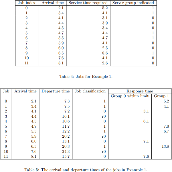
4.2 Example 1: n = 4, n0 = 2, n1 = 2 and Tlimit = 3.5
For this example, we assume that the system has n = 4 servers. Both Groups 0 and 1 have 2 servers each, i.e., n0 = n1 = 2. The service time-limit for Group 0 server is Tlimit = 3.5.
Table 4 shows the attributes of the jobs which will arrive at this system. Table 5 summaries the results of the simulation. The mean response time of the completed Group 0 jobs is 4/23.9 = 5.975 and the mean response time of the Group 1 jobs is 5/36.8 = 7.36.
4.3 Example 2: n = 4, n0 = 1, n1 = 3 and Tlimit = 3.5
This example is identical to Example 1 except that n0 = 1. Table 6 summaries the results of the simulation. The mean response time of the completed Group 0 jobs is 4/44.9 = 11.225 and the mean response time of the Group 1 jobs is 5/29.8 = 5.96. It is not surprising that the mean response time of the completed Group 0 jobs has gone up while that of Group 1 jobs has gone down. This is because in this example, there are fewer servers in Group 0.

5 Project description
This project consists of two main parts. The first part is to develop a simulation program for the system in Figure 1. The system has already been described in Section 3 and illustrated in Section 4. In the second part, you will use the simulation program that you have developed to solve a design problem.
5.1 Simulation program
You must write your simulation program in one (or a combination) of the following languages: Python 3 (note: version 3 only), C, C++, or Java. All these languages are available on the CSE system.
We will test your program on the CSE system so your submitted program must be able to run on a CSE computer. Note that it is possible that due to version and/or operating system differences, code that runs on your own computer may not work on the CSE system. It is your responsibility to ensure that your code works on the CSE system.
Note that our description uses the following variable names:
1. A variable mode of string type. This variable is to control whether your program will run simulation using randomly generated arrival times and service times; or in trace driven mode. The value that the parameter mode can take is either random or trace.
2. A variable time_end which stops the simulation if the master clock exceeds this value. This variable is only relevant when mode is random. This variable is a positive floating point number.
Note that your simulation program must be a general program which allows different param- eter values to be used. When we test your program, we will vary the parameter values. You can assume that we will only use valid inputs for testing.
For the simulation, you can always assume that the system is empty initially.
Hint: Do not write two separate programs for the random and trace modes because they share a lot in common. A few if–else statements at the right places are what you need to have both modes in one program.
5.1.1 The random mode
When your simulation is working in the random mode, it will generate the inter-arrival times and the workload of a job in the following manner.
1. We use {a1 , a2,..., ak,...,...} to denote the inter-arrival times of the jobs arriving at the dispatcher. These inter-arrival times have the following properties:
(a) Each ak is the product of two random numbers a1k anda2k, i.e ak = a1ka2k ∀k = 1, 2, ... (b) The sequence a1k is exponentially distributed with a mean arrival rate λ requests/s.
(c) The sequence a2k is uniformly distributed in the interval [a2l, a2u].
Note: The easiest way to generate the inter-arrival times is to multiply an exponentially distributed random number with the given rate and a uniformly distributed random number in the given range. It would be more difficult to use the inverse transform method in this case, though it is doable.
2. The workload of a job is characterised by two attributes: the server group (i.e., Group 0 or
1) that the job is to be sent to, and the service time of the job.
(a) The first step to determine which server group to send the job to. This decision is made by a parameter p0 ∈ (0, 1):
• Prob[a job is indicated by the user for a Group 0 server] = p0
• Prob[a job is indicated by the user for a Group 1 server] = 1 − p0
For example, if p0 is 0.8, then there is a probability of 0.8 that ajob is indicated for a Group 0 server and a probability of 0.2 for a Group 1 server. The server group for each job is independently generated.
(b) Once the server group for a job has been generated, the next step is to generate its service time. The service time distribution to be used depends on the server group.
i. If a job is indicated to go to a Group 0 server, its service time has the probability density function (PDF) g0 (t):

where

Note that this probability density function has 3 parameters: α0 , β0 and η0 . You can assume that β0 > α0 > 0 and η0 > 1.
ii. If a job is indicated to go to a Group 1 server, its service time has PDF:
where

Note that this probability density function has 2 parameters: α 1 and η 1 . You can assume that α 1 > 0 and η 1 > 1.
5.1.2 The trace mode
When your simulation is working in the trace mode, it will read the list of inter-arrival times, the list of service times and server groups from two separate ASCII files. We will explain the format of these files in Sections 6.1.3 and 6.1.4.
An important requirement for the trace mode is that your program is required to simulate until all jobs have departed from the system. You can refer to Table 2 for an illustration.
5.2 Determining the value of n0 that minimises a weighted mean re-sponse time
After writing your simulation program, your next step is to use your simulation program to de- termine the number of Group 0 servers n0 that minimises a weighted mean response time.
For this design problem, you will assume the following parameter values:
• Total number of servers: n = 10
• The service time limit Tlimit for Group 0 servers is 3.3.
• For inter-arrival times: λ = 3.1, a2l = 0.85, a2u = 1.21
• The probability p0 that a job is indicated for a Group 0 server is 0.74.
• The service time for a job which is indicated for Group 0: α0 = 0.5, β0 = 5.7, η0 = 1.9.
• The service time for a job which is indicated for Group 1: α 1 = 2.7 and η 1 = 2.5. The aim of the design problem is to minimise the weighted response time:
w0T0 + w1T1 (3)
where T0 is the mean response time of the completed Group 0 jobs and T1 is the mean response time of Group 1 jobs. The value of the weights w0 and w1 are fixed for this design problem, and they are given by 0.83 and 0.059 respectively. As an example, if T0 = 1.86 and T1 = 56.7, then the weighted mean response time is 0.83 × 1.86 + 0.059 × 56.7. The rationale behind choosing these weights is explained in Remark 3.
The aim of the design problem is to find the value of n0 to minimise this weighted response time. Note that we assume that there is at least a server in each group, therefore 1 ≤ n0 ≤ n − 1.
In solving this design problem, you need to ensure that you use statistically sound methods to compare systems. You will need to consider simulation controls such as length of simulation, number of replications, transient removals and so on. You will need to justify in your report on how you determine the value of n0 .
Remark 3 For the parameters above, out of all the jobs that are not re-circulated, 73.65% are Group 0 jobs within the time limit and 26.35% are Group 1 jobs. The average service time for Group 0 jobs within the time limit is 0.887 and that for Group 1 jobs is 4.5. The weights w0 and w1 ![]()
![]() . So the weights take into account the frequency of a class of jobs. We also use the inverse service time as a weight so that we are not giving too much advantage to Class 1 jobs as they have large service time requirement.
. So the weights take into account the frequency of a class of jobs. We also use the inverse service time as a weight so that we are not giving too much advantage to Class 1 jobs as they have large service time requirement.
2024-06-15