Hello, dear friend, you can consult us at any time if you have any questions, add WeChat: daixieit

ECON 23950: Economic Policy Analysis

Problem Set 1

1 Dynare Exercise

This is to get you started with Dynare, a powerful numerical tool that allows you to solve models, simulate policy experiments, and do a host of other exciting things you can’t do with a pen and paper!

1.  Set up your dynare environment by following the steps described in the dynare quick start guide.

2.  Open and examine the file “permg.mod” that computes the transition path of the economy to a permanent shock to government spending. It is useful to read pp.15-25 of the User Guide. Run the file by typing dynare permg.mod at the command prompt. If you get errors,  add the path by typing  addpath  c:\dynare\4.x.y\matlab where 4.x.y is the version number of Dynare.

3.  Run permg.m by typing permg. This is what happens to the economy over time when it is hit with a permanent shock to government spending.

4.  (This is the only question you need to turn in your work for.)  Let’s change the model a little bit. Suppose we rewrite the utility function such that

Redo the simulation by setting σ = 2. (Hint: You will need to add a parameter, rewrite the first line in the model, and modify the initial and end values.) Print out and turn in your code and impulse response diagrams. You are encouraged to rewrite the plotting code in matlab so that the graphs look prettier!

2    Two Ways to Model Government Spending

Consider an economy populated by many identical infinitely-lived households and many identical firms. The per period-utility of households is given by

u(Ct) = ln Ct.

with Ct being consumption at time t. Time is discrete and infinite:  t = 0, 1, 2, . . . ,.  The total utility of the household is then

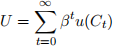
where β is the time discount factor (”patience” of households).

Consumers decide in each period how much to consume and save given their income. There is only one asset in this economy, capital Kt. The capital stock is owned by the household and evolves according to the following law of motion:

Kt+1 = It+ (1 − δ)Kt

where It  represents gross investment.

Firms are also owned by households. They use capital Kt  to produce (private) output with the production function

YtP  = Kt(α) .

The government has a predetermined sequence of public spending {Gt}∞t=0 to be paid solely with lump-sum taxes Tt. Assume that the government cannot borrow or save,  all its spending has to be financed each period.  In order for government expenditure to add to output, we assume the total output to consist of private and public output Yt  = YtP  + YtG, and where government output is given by YtG  = ϕGt.  where ϕ > 0.  Both private and public output are consumed by the households.

Part I.

1.  Considering that households pay lump sum taxes every period, write down its period-by- period budget constraint?

2. Use the law of motion for capital and the government budget constraint to replace It  and Tt  in the household budget.

3. Write down GDP Yt  as function only of Kt  and Gt  and plug the expression back into the budget constraint.

4.  Set up the household’s maximization problem.

5. Write down the first-order conditions for Ct  and Kt+1 .

6. Now consider a steady state with Ct  = Ct+1  = Css  and Kt  = Kt+1  = Kss.  Assume that government spending is constant over time at Gt  = G.  Use the first-order conditions to derive Kss.

7.  State the budget constraint in steady state and find Css  depending on Kss.  How does Css change with G?

8.  Does the government make households better off at steady state?  What does your answer depend on? Explain.

Part II.

Now suppose that government spending directly enters the utility function:

u(Ct, Gt) = ln Ct+ η lnGt

but household income is now only given by private consumption: Yt = YtP  = Kt(α).

1. How does the budget constraint look like now?  Write it again in a way so that it only depends on Ct, Kt, Kt+1 , and Gt  (besides given parameters).

2.  Set up the household problem and write down the first-order conditions.  Solve again for Css  and Kss.

3. Now imagine that the benevolent government tries to maximize the household utility at steady state. Write down the maximization problem. Notice that the household would still choose to consume and invest in a maximizing manner, which you derived in the previous questions.

4.  Solve the  maximization problem for the government. It may be convenient to define X ≡ Kss(α) − δKss.

5. Explain your answer intuitively. How does the optimal policy depend on η and X? Explain intuitively.

3    Fiscal Multiplier with Proportional Taxes

Imagine an economy similar to the one we discussed in class with proportional taxes this time. The household, taking as given the initial bond holding b0  and the fiscal policy, maximizes the lifetime utility

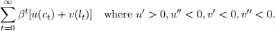
with respect to a sequence of bond holding bt+1, labor effort lt, and consumption ct  subject to

Yt+ (1 + rt)bt = ct+ bt+1 + τtYt     ∀t

where

Yt = f(lt)   where f′  > 0, f′′  < 0.

The government levies a proportional income tax to run balanced budget at each period:

Gt = Tt = τtYt ∀t

1. Assuming that the household takes {Gt}∞t=0 as given (Do not replace Gt with τtYt yet), solve the household’s maximization problem to derive the intratemporal optimality condition.

2.  Derive the economy-wide resource constraint.

3.  Can consumption and labor be solved contemporaneously for each period? Why?

4.  Draw a diagram with labor on x-axis and consumption ony-axis to illustrate what happens to the optimal allocation when τ rises. Explain intuitively.  You may want to compare your result to the one we did in class with lump-sum taxes.

5.  (Bonus Question) Using the implicit differentiation technique, can you derive and sign τ(l)t(t) ?

Explain.

6.  Suppose u(c) = lnc;  v(l) = ln(1 − l);  f(l) = lα .  Solve explicitly for the optimal labor and consumption allocation. Does a tax cut stimulate the economy? Explain.

4    Tax Incentive for Investment

In the infinite period model we studied in class, we have seen that when the government taxes output produced using capital, we get distortions.  Here, we will analyze what happens at steady state when the government exempts investment from taxation (thus making the tax effectively a consumption tax).

The economy can be summarized as consisting of an infinitely-lived representative household that maximizes the following total utility function:

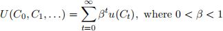
with production technology

Yt = Ktα , where 0 < α < 1

There is no government production, so all tax proceeds are burned (ϕ = 0). The law of motion for capital accumulation is

Kt+1 = (1 − δ)Kt + It , where 0 < δ < 1

So far,  everything  is  the same  as the model we discussed in class.   However,  investment  is excluded from taxation, so that the budget constraint is

Yt = Ct+ It+ τ(Yt − It).

1.  Show that this taxation scheme effectively corresponds to a consumption tax, i.e.  show that you can write the budget constraint as

Yt = (1 + τc)Ct + It.

Express τc  as a function of τ .

2.  Set up the optimization problem of the representative household, calculate the first-order conditions, and derive the Euler equation.

3. Assume that the economy is at a steady-state where the capital stock stays at Kss. Cal- culate the steady-state levels of capital, Kss, and consumption, Css, as a function of the model’s parameters and τc.

4.  Does taxation distort the capital stock in the long-run?

5.  Does taxation crowd out consumption in the long-run?

6.  Calculate the steady-state levels of investment, Iss, output, Yss, and the government rev- enue, Gss  as a function of the model’s parameters and τc.

7.  Graph Gss  as a function of τc. Does this tax system exhibit a Laffer curve? Explain.