Submit: Monday, 2020-February-25 before 11:45ET

Please submit your solutions on Blackboard in a single PDF file that includes all math and numerical results. Only the contents of this PDF will be graded.

For control purposes, please also provide any code you write to solve the questions in one of the following ways:

1. Include all of your code in the PDF as an appendix.

2. In the PDF provide a link to your online code repo where the code resides.

This is a graded assignment and the entirety of your submission must contain only your own work. Do not make your code repo public until after the submission deadline. If people find your code and use it to solve questions, we will consider it cheating for all parties involved. You may benefit from publicly available literature including software (that is not from classmates), as long as these sources are properly acknowledged in your submission.

Copying math or code from each other is clearly not allowed and will be considered as academic dishonesty. Discussing with the instructor and the teaching assistant to get clarification, or to eliminate doubts is acceptable.

By submitting a PDF file in response to this take home assignment you are declaring that the contents of your submission, and the associated code is your own work, except as noted in your acknowledgement citations to resources.

Start early and use the office periods well. The office periods are on gcal and contain hangout links for remote participants to our class. You may call 1-617-3733021 to reach Deniz to request a video meeting at the office periods.

It is your responsibility to provide the necessary and sufficient evidence in the form of math, visualizations, and numerical values to earn scores. Do not provide a minimal set of what you interpret is being precisely requested; you may be providing too little evidence of your understanding. On the other hand, also please do not dump in unnecessarily large amounts of things; you may be creating the perception that you do not know what you are doing. Be intentional in what you present and how you present it. You are trying to convince the reader (grader) that your mathematical design, code implementations, and generated results are legitimate and correct/accurate.

Question 1 (35%)

The probability density function (pdf) for a 2-dimensional real-valued random vector X is as follows: p(x) = P(L = 0)p(x|L = 0)+P(L = 1)p(x|L = 1). Here L is the true class label that indicates which class-label-conditioned pdf generates the data.
The class priors are P(L = 0) = 0.9 and P(L = 1) = 0.1. The class class-conditional pdfs are p(x|L = 0) = g(x|m 0 ,C 0 ) and p(x|L = 1) = g(x|m 1 ,C 1 ), where g(x|m,C) is a multivariate Gaussian probability density function with mean vector m and covariance matrix C. The parameters of the class-conditional Gaussian pdfs are:

For numerical results requested below, generate multiple independent datasets consisting of iid samples drawn from this probability distribution; in each dataset make sure to include the true class labels for each sample. Save the data and use the same data set in all cases.
• consists of 10 samples and their labels for training;
• consists of 100 samples and their labels for training;
• consists of 1000 samples and their labels for training;

• consists of 10000 samples and their labels for validation;

Part 1: (5/35) Determine the classifier that achieves minimum probability of error using the knowledge of the true pdf. Implement this minimum-P(error) classifier and use it on D 10K validate to draw an estimate of its ROC curve on which you mark the minimum-P(error) classifier’s operating point. Specify the classifier mathematically, present its ROC curve and the location of the min-P(error) classifier on the curve, an estimate of the min-P(error) achievable (using counts of decisions on D 10K validate ). As supplementary visualization, generate a plot of the decision boundary of this classification rule overlaid on the validation dataset. This establishes an aspirational performance level on this data.

Part 2: (15/35) With maximum likelihood parameter estimation technique train three separate logistic-linear-function-based approximation of class label posterior functions given a sample. For each approximation use one of the three training datasets D 10 train , D 100 train , D 1000 train . When optimizing the parameters, specify the optimization problem as minimization of the negative-log-likelihood of the training dataset, and use your favorite numerical optimization approach, such as gradient descent or Matlab’s fminsearch. Determine how to use the class-label-posterior approximation to classify a sample, apply these three approximations of the class label posterior function on samples in D 10K validate , and estimate the probability of error these three classification rules will attain (using counts of decisions on the validation set). As supplementary visualization, generate plots of the decision boundaries of these trained classifiers superimposed on their respective training datasets and the validation dataset.

Part3: (15/35)Repeattheprocessdescribedinpart2usingalogistic-quadratic-function-based approximation of class label posterior functions given a sample.

Note 1: With x representing the input sample vector and w denoting the model parameter vector, logistic-linear-functionreferstoh(x,w)=1/(1+e −w

T z(x) ), wherez(x)=[1,x T ] T ; andlogisticquadratic-function refers to h(x,w) = 1/(1+e −w T z(x) ), where z(x) = [1,x 1 ,x 2 ,x 2 1 ,x 1 x 2 ,x 2 2 ] T .

Question 2 (30%)

We have two dimensional real-valued data (x,y) that is generated by the following procedure,
where all polynomial coefficients are real-valued and v ∼ N (0,σ 2 ):

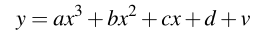
Let w = [a,b,c,d] T be the parameter vector for this polynomial relationship. Given the knowl- edge of σ and that the relationship between x and y is a cubic polynomial corrupted by additive noise as shown above, iid samples D = {(x 1 ,y 1 ),...,(x N ,y N )} generated by the procedure using the true value of the parameters (say w true ), and a Gaussian prior w ∼ N (0,γ 2 I), where I is the 4×4 identity matrix, determine the MAP estimate for the parameter vector.

Write code to generate N = 10 samples according to the model; draw iid x ∼Uniform[−1,1] and choose the true parameters to place the real roots (for simplicity) for the polynomial in the interval [−1,1]. Pick a value for σ (that makes the noise level sufficiently large), and keep it constant for the experiments. Repeat the following for different values of γ (note that as γ increases the MAP estimates approach the ML estimate).

Generate samples of x and v, then determine  the corresponding values of y. Given this particular realization of the dataset D, for each value of γ, find the MAP estimate of the parameter vector and calculate the squared L 2 distance between the true parameter vector and this estimate.

For each value of γ perform at least 100 experiments, where the data is independently generated according to the procedure, while keeping the true parameters fixed. Report the minimum, 25%, median, 75%, and maximum values of these squared-error values, , for the MAP estimator for each value of γ in a single plot. How do these curves behave as this parameter for the prior changes?

Note: Make sure to change gamma to cover a sufficiently broad range to see its effects at multiple scales. To achieve this, you might want to select values for this hyperparameter as power of 10 linearly spaced from −B to +B, so that you cover the interval  logarithmically. Choose B > 0 well.

Question 3 (35%)

Select a Gaussian Mixture Model as the true probability density function for 2-dimensional real-valued data synthesis. This GMM will have 4 components with different mean vectors, differ- ent covariance matrices, and different probability for each Gaussian to be selected as the generator for each sample. Specify the true GMM that generates data.

Conduct the following model order selection exercise multiple times (e.g., M =100), each time using cross-validation based on many (e.g., at least B = 10) independent training-validation sets generated with bootstrapping.

Repeat the following multiple times (e.g., M = 100):

Step 1: Generate multiple data sets with independent identically distributed samples using this true GMM; these datasets will have, respectively, 10, 100, 1000 samples.

Step 2: (needs lots of computations) For each data set, using maximum likelihood parameter estimation with with the EM algorithm, train and validate GMMs with different model orders (using at least B = 10 bootstrapped training/validation sets). Specifically, evaluate candidate GMMs with 1, 2, 3, 4, 5, 6 Gaussian components. Note that both model parameter estimation and validation performance measures to be used is log-likelihood of the appropriate dataset (training or
validation set, depending on whether you are optimizing model parameters or assessing a trained

model).

Step 3: Report your results for the experiment, indicating details like, how do you initialize your EM algorithm, how many random initializations do you do for each attempt seeking for the global optimum, across many independent experiments how many times each of the six candidate GMM model orders get selected when using different sizes of datasets... Provide a clear description of your experimental procedure and well designed visual and numerical illustrations of your experiment results in the form of tables/figures.

Note: We anticipate that as the number of samples in your dataset increases, the cross- validation procedure will more frequently lead to the selection of the true model order of 4 in the true data pdf. You may illustrate this by showing that your repeated experiments with different datasets leads to a more concentrated histogram at and around this value.