Hello, dear friend, you can consult us at any time if you have any questions, add WeChat: daixieit

MATH237: Calculus 3

Written Assignment 4

Fall 2021

Instructions

● There are five submission slots on Crowdmark: Q1, Q2, Q3 and Q4. Please upload your solutions into the appropriate slots.

● Don’t forget about the LATEX Bonus and the opportunity to earn up to +2% on your final course grade. See LEARN → Activities and Assignments → Written Assignments and scroll down to ‘LaTeX Bonus’ for more info.

● For Q1, your sketches may either be hand-drawn or graphed with software. You may submit them as separate image files on Crowdmark, or you may insert them alongside the rest of your write-up. If you’d like to do the latter, a code snippet is provided in the .tex template. [If you submit as separate image files, you will still be eligible for the LaTeX bonus.]

Problems

Q1. Let f : R² → R be given by f(x, y) = 2x³ − 3x² + y² − 2y.

(a) Find the critical points of f and classify them into local maxima/minima and saddle points.

(b) Let D be the region in the xy-plane that lies inside the quadrilateral with vertices at (0, 0), (2, 0), (2, 2) and (1, 2), together with its boundary edges. Sketch D.

(c) Find the global maximum and minimum values of f on D and the points at which they occur. Mark these points on your sketch of D.

Q2. Consider the lines L1 and L2 in R³ given by the vector equations

(a) Find an expression for the distance between two points on L1 and L2. Your expression should be a function f : R² → R.

(b) By finding the extreme values of f, find the shortest distance between L1 and L2. Be sure to fully justify your answer.

[Hint: The expression for the distance-squared is often simpler than the expression for the distance. So you may find it easier to work with f² instead of f. If you do so, be sure to clearly explain how the process of optimizing f² is related to optimizing f.]

Q3. The Cauchy–Schwarz inequality says that if = (a1, . . . , an) and = (b1, . . . , bn) are two vectors in Rⁿ, then

In this exercise you will give a proof of this inequality using multivariable calculus.

(a) Assume that the inequality is true for all ∈ Rⁿ with . Deduce from this that the inequality must then be true for all  ∈ Rⁿ.

(b) Find the maximum and minimum values of the function  subject to the constraint where is a fixed positive real number.

[Hint: The Lagrange multipliers algorithm applies in the same way to a function of n variables as it does to functions of 2 or 3 variables. You may use, without proof, the fact that the set is closed and bounded and has no “edge points.”]

(c) Using your findings in parts (a) and (b), give a proof of the Cauchy–Schwarz inequality.

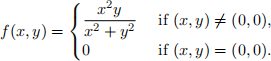
Q4. Let be a unit vector in R² and let f : R² → R be defined by

(a) Find .

(b) Using your solution to (a), find ∇f(0, 0).

(c) Use the Lagrange multipliers algorithm to find the maximum and minimum directional derivatives at (0, 0). [Hint: What are you trying to optimize? What is the constraint?]

(d) If you’ve solved (b) and (c) correctly, you will have found that the maximum and mini-mum directional derivatives are not equal to and . This appears to contradict the Greatest Rate of Change Theorem given in Unit 7.2. What went wrong?

Explain.