Hello, dear friend, you can consult us at any time if you have any questions, add WeChat: daixieit

MATH6173 Statistical Computing — Coursework 1

Instructions for Coursework 1

1. This coursework assignment is worth 50% of the overall mark for the module MATH6173.

2. Your completed work must be submitted electronically via Blackboard.

3. Your submission must consist of exactly one written report including the answers and any tables and graphs to the questions in Section 1: R Programming Part I, together with one R script file containing all the R code you used to obtain your results for questions in both Section 1 and Section 2. In the R script, you must use comments to make it clear to which questions the R codes are answering.

4. Your written report should be in pdf format. Please name your report report as <your student ID>.pdf. For example, if your student ID is 12345678, then your report must have the filename 12345678.pdf.

5. Your R script file must have the filename <your student ID>.R. For example, if your student ID is 12345678, then your script must have the filename 12345678.R.

6. Your entire R script file should be reproducible and run without any errors.

7. You must present elegant and informative plots in the written report, including the use of appropriate plotting area, points/lines sizes and colours. Also please include meaningful labels, titles and legends.

8. You must informatively comment your R code including indicating where each question and task begins.

9. You must not load any add-on packages, e.g. using function library or require.

10. The standard Faculty rules on late submissions apply: for every weekday, or part of a weekday, that the coursework is late, the mark will be reduced by a factor of 10%. No credit will be given for work which is more than one week late.

11. All coursework must be carried out independently. You are reminded of the University’s Academic Integrity Policy, see https://www.southampton.ac.uk/quality/assessment/academic_integrity.page.

12. In the interests of fairness, queries which relate directly to the coursework must be made via the MATH6173: Coursework 1 Discussion Forum on Blackboard. This ensures that everybody has access to the same information.

Section 1: R Programming Part I

Question 1. Two-sample testing

[22 marks]

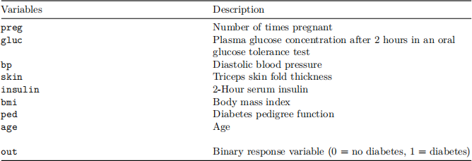
The dataset in the file diab.txt is originally from the US National Institute of Diabetes and Digestive and Kidney Diseases and contains measurements from n = 768 female individuals. The data contains a series of eight measurements variables, and a response variable indicating whether or not a patient has diabetes. The variables in the dataset are described in following table.

(a) [2 marks] Import the dataset from the file diab.txt into your own work space. Calculate the following quantities:

● number of patients that have diabetes, and number of patients that do not have diabetes

● median age of patients

● mean body mass index for patients that have diabetes, and mean body mass index for patients that do not have diabetes

(b) [2 marks] Produce a side by side boxplot to show the distributional information of all the eight measurements after scaling (subtracting the mean and dividing by the standard deviation).

(c) [2 marks] We want to test whether the mean value of body mass index (BMI) are the same between patients with diabetes and patients without diabetes. Let us use Student’s t-test here and assume the variances of BMI in both groups are equal. List your null and alternative hypotheses, perform your test and give the p-value. Do you reject your null hypothesis at the significance level of 0.05?

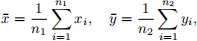
(d) [6 marks] Suppose now we want to write our own code to perform a similar test in (c) without assuming equal variance. To achieve this, we can use the Welch’s t-test. Suppose we have two independent groups of random variables x1, . . . , xn1 and y1, . . . , yn2 . We define their sample means as:

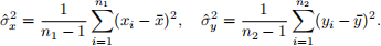
and their sample variances as:

Then we can define the unbiased variance estimator as:

Therefore, we obtain

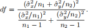
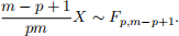
which is the so-called Welch’s t-test statistic. Under the null hypothesis of mean equality, we have the distribution of this test statistic can be approximated by a Student’s t-distribution with degrees of freedom

Write your own code to calculate the Welch’s t-test statistic for the same hypothesis testing problem in (c). Give the value of this test statistic, the degrees of freedom, and the p-value of your test. Do you reject the null hypothesis at the significance level of 0.05?

(e) [3 marks] The F-distribution is a continuous probability distribution that arises frequently in probability theory and statistics. It has two parameters, and we write if a random variable X follows from a F-distribution with parameters d1 and d2. You can use the R functions df, pf, qf and rf to obtain the probability density function, cumulative distribution function, quantile function and random generation function of F-distribution. Read the help file of above functions and produce the following four plots in one page with 2 × 2 layout.

● plot 1: probability density function of F8,10.

● plot 2: cumulative distribution function of F8,10.

● plot 3: a probability histgram for 100 independently generated random numbers from F8,10.

● plot 4: empirical density function of the same 100 random numbers in plot 3.

(f) [7 marks] Suppose now we want to simultaneously test if the mean values of all the eight measurements are equal between patients that have diabetes and patients that do not have diabetes. To achieve this, we can use the Hotelling’s T-squared test, which is a natural generalizations of the Student’s t-test to multivariate hypothesis testing. Suppose we have two independent groups of random p-vectors x1, . . . , xn1 and y1, . . . , yn2 (all the vectors are p-dimensional). We define the their sample mean vectors as:

and their sample covariance matrices as:

Then we can define the unbiased pooled covariance matrix as:

Therefore, we obtain

which is the so-called Hotelling’s two-sample T-squared statistic. If we further assume that both groups consists of observations that are identically and independently drawn from multivariate normal distribution N(µ, Σ), then

where T2(p, n1 + n2 − 2) denotes the so-called Hotelling’s T-squared distribution with parameters p and n1 + n2 − 2. If a random variable X has a Hotelling’s T-squared distribution, i.e., we have

Let group 1 be the eight measurements for all the patients with diabetes, and let group 2 be the eight measurements for all the patients without diabetes. List your null and alternative hypotheses. Write your own code to calculate the Hotelling’s two-sample T-squared statistic, derive the p-value of your test. Do you reject your null hypothesis at the significance level of 0.05?

        Hints:

(1) In hypothesis testing, the p-value is defined as the probability of obtaining test statistics at least as extreme as the results actually observed, under the assumption that the null hypothesis is true.

(2) Observe the Hotelling’s two-sample T-squared statistic, if the mean difference between two groups is small (then  should be close to 0), the value of T2 will tend to be small. Otherwise if the mean difference between two groups is large, the value of T2 will tend to be large as well.

Question 2: Non-parametric kernel density estimation

[28 marks]

Density estimation is the problem of reconstructing the probability density function (pdf) from a set of given data points. Namely, we observe X1, . . . , Xn and we want to estimate the underlying unknown pdf, denoted by f(x), generating this dataset, which is one of the central topics in (non-parametric) statistical research.

The so-called kernel density estimator (KDE) is one of the most famous method for this problem. Here we give a formal definition of the KDE in the following formula:

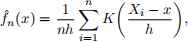
where (x) is the empirical estimation of the true pdf f(x), K(·) is called the kernel function that is generally a smooth, symmetric function, and h > 0 is called the bandwidth that controls the amount of smoothing in the estimation.

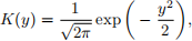
(a) [5 points] Consider the Gaussian kernel function:

where exp(·) is the exponential function. First, generate 200 random numbers from N(0, 1) distribution as your dataset. Next, write your own code to estimate the pdf of N(0, 1) from the dataset, i.e., calculate (x) for x being a vector of equally spaced 250 points on [ −4, 4] with h = 0.3. Please present your calculated (x) and the true pdf f(x) of N(0, 1) on the same plot, and show this plot on your report.

(b) [10 points] There are many other forms of kernel functions, for example:

● Uniform:

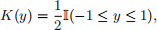
● Epanechnikov:

where I(·) is the indicator function. Now write a function mysimpleKDE with the following features:

● Arguments

(1) data is a numeric vector containing the data that we want to estimate the pdf from.

(2) h is a numeric object specifying the bandwidth of the kernel function.

(3) kernel is a character object specifying the kernel function we want to use, by default it is “gaussian”, and we can also set it to be “epanechnikov” or “uniform”.

(4) range is a two-variate numeric vector specifying the starting point and end point of an interval of x on which we want to estimate the density.

● Computation

– Calculate (x) for x being a vector of equally spaced 250 points on the interval specified by range.

● Return

– A list containing the following elements:

(1) density is a numeric vector corresponding to the empirical probability density value for each data point.

(2) kernel is a character object corresponding to the type of kernel function we used in the estimation. It should be either “gaussian”, “epanechnikov” or “uniform”.

(c) [5 points] Generate 50 random numbers from N(1, 1). Use your function mysimpleKDE and multiple for-loops to produce a 3 × 3 plots, each on appropriate x-range, showing (x) with combinations of three different kernel functions and different values of h ∈ {0.1, 0.3, 0.5}.

(d) [8 points] In practice, we should carefully select h to minimise the asymptotic mean square error (AMSE) of density estimation. Let us fix the kernel function to be “gaussian”. Repeatedly generate 200 random numbers from N(0, 1) distribution for 100 times. In each time j we can calculate the KDE (x) at x for different values of bandwidth h, where h is from the set {0.1, 0.15, 0.2, . . . , 1}. The corresponding averaged mean squared error for each h can be approximated as:

Here again we fix x = (x1, . . . , xm)T being a vector of equally spaced 250 points on [ −4, 4]. Calculate (h) for different values of h and show them in the report. What is the optimal value of h based on your results?

        Hints:

(1) You can use the function seq to generate equally spaced points in a certain range.

(2) You may find the element-wise maximum function pmax and element-wise and operator & helpful.

(3) You will need to use for-loops and conditional statements in this question.

Section 2: R Programming Part II

Question 1: Multivariate distribution

[13 marks]

If a p-dimensional random vector X is distributed according to a multivariate normal distribution (MVN), then we write X ~ MVN(µ, Σ), where µ is the p-dimensional mean vector and Σ is the p × p variance-covariance matrix. The probability density function of an MVN is given by

(a) [8 marks] Write a function calcLogMVN that calculates the natural logarithm of the joint probability density for any number of MVN random variables from the same p-dimensional MVN distribution. The calcLogMVN function have the follwoing features.

Arguments:

(1) xMat is a numeric matrix, where the rows are independent random variables of a p-dimensional MVN distribution.

(2) mu is a numeric vector representing µ in equation (1).

(3) Sigma is a numeric matrix representing Σ in equation (1).

Computation:

● Without using the %*% operator, the calcLogMVN function calculates the natural logarithm of the joint density of the random variables in xMat given mu and Sigma according equation (1).

Return:

● A numerical value as calculated in Computation.

IMPORTANT: Heavy penalties will be applied if the following requirements are not met for this question.

● You must not use any existing functions that already calculate the density of an MVN.

● For matrix multiplications, you must only use loops and operators/functions for scaler addition and multiplication.

(b) [3 marks] For the calculations to be feasible in part (a), the arguments have certain restrictions.

● mu is a numeric vector with a length of p, which is the number of columns of xMat.

● Sigma is a squrare matrix.

● The numbers of rows and columns of Sigma must both equal to the length of mu.

Add additional R commands at the beginning of your calcLogMVN function in part (a) to check that valid inputs have been provided. If invalid inputs are passed to this function, then it will stop prematurely along with an apporpriate error message.

(c) [2 marks] Use the function created in part (a) & (b) to calculate the natural logarithm of the joint density of the random vectors X1 = (−1.00,0.10, 0.80), X2 = (−0.50, −0.10, 1.25) and X3 = (−1.20, −0.50, 0.75) under the distribution MVN(µ, Σ) with

Question 2: Integration by the trapezoidal rule

[17 marks]

Figure 1 shows the cubic polynomial

f(x) = (x + 3)(x − 1)(x − 2.5).

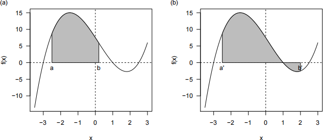
Figure 1: f(x) = (x + 3)(x − 1)(x − 2.5). In panel (a), the area shaded in grey is the area between f(x) and the x-axis within the x-interval [a, b], while the shaded region in panel (b) is the area between f(x) and the x-axis within the x-interval [a0 , b0 ]

.

When a curve f(x) is above the x-axis for the x-interval [a, b] as in Figure 1 (a), we can calculate the area between f(x) and the x-axis within [a, b] using the trapezoidal rule for integration:

with subintervals defined by a = x0 < ... < xN = b.

(a) [10 marks] Write a function calcArea that calculates the area between the curve in equation (2) and the x-axis for any given x-interval [a, b].

Arguments:

(1) xVec is a numeric vector with elements corresponding to x0, ..., xN in equation (3). Note: You can assume that for marking, the x-intercepts will not fall within any of the subintervals; however, the subintervals are allowed to have different lengths. The x-intercepts are the values of x that give f(x) = 0.

Computation:

● This function calculates the area between the x-axis and the cubic polynomial in equation (2) according to the trapezoidal rule with subintervals defined by xVec.

Hint: Multiply by -1 for the part(s) of the curve with f(x) < 0.

Return:

● A numerical value which is the area as calculated in Computation.

(b) [5 marks] Write a function calcAreaGen that generalises the calcArea function in part (a):

● The calcAreaGen function have additional numeric arguments s, u, v and w, which corresponds to the parameters of the cubic polynomial f(x) = s(x − u)(x − v)(x − w).

● The calcAreaGen function calculates and returns the area between the x-axis and f(x) = s(x − u)(x − v)(x − w).

(c) [2 marks] Use the function calcAreaGen created in part (b) to calculate the area between the x-axis and f(x) = 0.25(x+5)(x+1.5)(x−0.5), using the sequence a = x0 = −5.5 < −5.4 < ... < 0.9 < 1.0 = xN = b to define the subintervals. In this case the subintervals all have the same length of 0.1.

IMPORTANT: You must use loops for this question, otherwise a heavy penalty will be applied.

Question 3: Finding a set of unique paths

[20 marks]

A path in two dimensional space is a line that has a starting point at (x, y)-coordinates of (xo, yo) and an end point at (xe, ye). In this question, you can assume that xo ≤ xe.

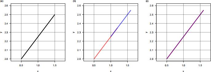
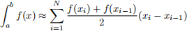
Figure 2: Examples of paths in two dimensional space. (a) A path with a starting point at (xo, yo) = (0.5, 2) and end point at (xe, ye) = (1.5, 2.5). (b) Two overlapping paths. The red path has a starting point at (0.5, 2) and end point at (1.2, 2.35), while the blue path has starting and end points at (1.0, 2.25) and (1.6, 2.55) respectively. (c) The path formed by merging together the red and blue paths in (b).

(a) [5 marks] Write a function getYIntAndSlope, which calculates the y-intercept and the slope of a path. Thus, the function will have the following features.

Arguments:

● xo is a numeric object representing the x-coordinate of the starting point (xo) of a path,

● yo is a numeric object representing the y-coordinate of the starting point (yo) of a path,

● xe is a numeric object representing the x-coordinate of the end point (xe) of a path, and

● ye is a numeric object representing the y-coordinate of the end point (ye) of a path.

Computations:

● This function calculates the y-intercept and the slope of the path given by the starting and end points as specified by the arguments.

Returns:

● A numeric vector, where its first element is the y-intercept and the second is the slope. Note: the y-intercept and slope in the vector must be in that order.

(b) [15 marks] Write a function getPathSet that extracts the unique set of paths. Specifically, it would have the following features.

Arguments:

(1) pathMat is a numeric matrix with four columns. Each row specifies a path in two dimensional space, while the columns specify the following information.

● column 1: the x-coordinate of the starting point (xo),

● column 2: the y-coordinate of the starting point (yo),

● column 3: the x-coordinate of the end point (xe), and

● column 4: the y-coordinate of the end point (ye).

For example, if the path in Figure 2 (a) is in pathMat, then the row corresponding to that path should look like 0.5 2.0 1.5 2.5.

Computation:

● This function extracts the unique paths in pathMat.

● Overlapping paths are replaced with a single path formed by merging those paths together. For example, in Figure 2 (b) there are two overlapping paths in red and blue. They should be merged into one path (purple) as in panel (c). The purple path should be added to the output matrix, while the red and blue paths are excluded.

Hint: Use the getYIntAndSlope function in part (a) as part of the computation.

Return:

● A numeric matrix with four columns.

– The rows represent the set of unique paths generated in Computation.

– The columns of the vector are the (x,y)-coordinates of the starting and end points of those paths, and the order of the columns are the same as in the argument pathMat.

IMPORTANT:

● You must use loop(s) and conditional statements for part (b) of this question, otherwise a heavy penalty will be applied.

● You will only obtain marks for part (b) of this question if your function produces a matrix with the correct set of paths.