Hello, dear friend, you can consult us at any time if you have any questions, add WeChat: daixieit

Computer lab 1 for Busstat 2. Correlation and Regression.

Computer lab 1 consists of a number of questions to be solved with SPSS. It is important that the “Instructions for lab reports in Statistics” is followed. The reports should be written in groups of two or three students (in some special cases students can be allowed to write the report alone). It is strictly forbidden to copy other reports (i.e. you are not allowed to write the report in a group of for example 10 students and then make five copies. All reports should be original). The lab report should be handed in on Canvas. The deadline is 24/11, 15.00.

1. The file Stock.sav contains data of mean and standard deviation of excess return of the S&P 50 stocks. Examine the relation between the two variables graphically by using a scatter plot. Calculate the correlation between two variables.

a. Comment on the relationship. Is the relationship strong?

To make a scatter plot in SPSS go to “Graphs” → “Legacy Dialog” → “Scatter/Dot”. Choose “Simple scatter” and click Define. Move one of the variables of interest to the Y-axis field and the other variable of interest to the X-axis field. It does not matter which variable you put on which axis. Then click ok. The scatter plot appears in the output window. To calculate simple correlations in SPSS, go to “Analyze” → “Correlate” → “Bivariate”. Highlight the variables of interest and move them to the variables box. Then click OK. The estimated correlations then appear in the output window.

2. The file Stock.sav contains data of mean and standard deviation of excess return of the S&P 50 stocks. In finance the relationship between excess return (defined as the return minus the return of a risk free alternative) is important. The assumption is that a higher risk measured as a higher standard deviation should lead to a higher excess return to compensate for the risk. One way to model this relationship is via the following simple linear regression model:

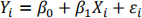
where Yi is the mean excess return for company i and Xi is the standard deviation of the excess return

a. Test the hypothesis versus (you may decide α=0.1, 0.05 or α=0.01 yourself). Comment the conclusion of the test. Is it in line of what you expected? Also comment on the sign of . Is the sign what you expected?

b. Interpret and comment on the R-square of the model.

To calculate sample regression parameters and the variance estimates in SPSS, go to “Analyse” → “Regression” → “Linear”. Then highlight your dependent variable and move it to the ‘’dependent” window. Next highlight your independent variable and move it to the ‘’independent” box and click OK. All relevant output then appears in the output window.

3. In Fair (1978, A Theory of Extramarital Affairs. Journal of Political Economy, 86, 45–61) it was investigated what factors that determine if a partner has an extramarital affair. In the paper the author uses regression analysis and in this question we will use the same data (Affairs.sav). It consists of 601 observations and we will estimate the following model:

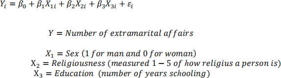
The file “Affairs.sav” contains data. Use this data to answer the following:

a. Test the hypothesis against the alternative hypothesis 0H : at least some is non-zero at significance level 0.1. Based on your test, do you think the model is useful for predictions of extramarital affairs?

b. Test if education have a significant effect on extramarital affairs (i.e. test if is significantly different from 0) at significance level 0.1.

c. By checking the histogram, the residuals do not appear to be normally distributed. Is that a problem here? Motivate.

To calculate multiple regression parameters and the variance estimates in SPSS, go to “Analyze” → “Regression” → “Linear”. Then highlight your dependent variable and move it to the ‘’dependent” window. Next highlight your independent variables and move them to the ‘’independent” box. Furthermore, we need to get the residuals. Click on the save button and select residuals/unstandardized and click “continue”. Finally, click the OK button. All relevant output then appear in the output window, except the residuals that appear as a new variable in the data window. Then in order to get a histogram go to “Graphs” → “Legacy Dialog” → “Histogram”. Then highlight the variables of interest and move them to the variables box in the box that pop-up.

4. A professor at the department of Economics hates animals. He is convinced that pigs are the major source of emissions that destroys ozone. Therefore the professor wants to investigate the impact of pigs on the ozone. However, the professor gets some comments at a seminar and he is told that he also needs to include the variable population in the regression model. In the dataset ozone.sav you find data for ozone, pigmeat produced and population. In this question you should estimate a simple linear regression models where the variable pigmeat is the only independent variable and the ozone variable is the dependent variable. Then estimate a second multiple linear regression model where pigmeat and population are the independent variables and the ozone variable is the dependent variable. Finally save the unstandardized residuals from the multiple linear regression model and make a scatterplot where the unstandardized residuals from the multiple linear regression model is on the Y-axis and the variable pigmeat is on the X-axis.

a. Comment on the difference between the estimated coefficients for the pigmeat variable for the simple linear regression model and the multiple linear regression model. Do you reject the null hypothesis that pigmeat does not have an effect on the ozone in both models? Why do you observe a difference regarding the pigmeat variable in both models?

b. By looking at the scatterplot, does the variance of the error term look constant or not?

c. What is the consequence for the hypothesis testing (t-tests and F-tests) if one finds that the variance of the error term is non-constant?