STAT 231 Fall 2021 Coursework 4
Hello, dear friend, you can consult us at any time if you have any questions, add WeChat: daixieit
STAT 231 Fall 2021 Coursework 4
Assignment Component
You may create your document in Word, Google Docs, LaTeX or any other word processor. The requirement to type your assignment is to facilitate the marking of hundreds of assignments so that the marked assignments can be returned to you in a timely fashion. It is also useful for you to gain some experience in creating a document containing mathematical expressions. Two documents have been posted in the Assignment 1 folder in LEARN on how to use the equation editor in Word. If you wish to use LaTeX then you may find Overleaf particularly useful for this. See https://www.overleaf.com/edu/uwaterloo
Upload your assignment component to Crowdmark as a pdf file for marking. You can upload your assignment as one document or individually for each problem. If you upload one document then you must drag and drop the pages for each problem to the appropriate question as indicated in Crowdmark. You can resubmit your assignment any number of times before the due time. Therefore, to ensure that there are no issues with uploading we advise you to upload your assignment well in advance of the due time. Assignments which are left as a single document and not uploaded to the appropriate places in Crowdmark will be assigned a 10% penalty.
In addition to submitting your assignment component to Crowdmark, you must submit your assignment as a single pdf document to the Assignment 4 LEARN Dropbox to facilitate the running of your assignment through plagiarism detection software.
Many problems on this assignment indicate that your written answers must be given in sentences. An overall penalty of 5% is applied to assignments which do not follow these instructions.
In this assignment you are asked to use R to answer some problems. The answers/results you obtain using R must be included in your Crowdmark pdf submission. Additionally, the R code that you use must be uploaded as an R file to the appropriate LEARN Dropbox. You should not include your R code in your Crowdmark submission.
Effectively commenting your code is a really important skill to develop. Markers will review your file and run it to verify the answers match those in your Crowdmark submission and that the code runs without error. Your code must correctly find the answers needed to get the marks associated with the problems. Good commenting will allow the marker to more easily assign you a full score when reviewing your file. Please ensure your code submitted in the R file is well commented.
Checklist to complete for this assignment:
Upload the pdf of your assignment component of Coursework 4 to Crowdmark by the deadline. A penalty of 5% per hour is applied for late assignments.
Upload your assignment component of Coursework 4 as a single pdf document to the appropriate LEARN Dropbox by the deadline.
Upload the R file of your assignment component to the appropriate LEARN Dropbox by the deadline. A penalty of 10% is applied if the R file is uploaded late or is missing.
If you have not already done so, upload your data set to the appropriate LEARN Dropbox.
This assignment is based on the material in Chapters 1-4 and Sections 5.1-5.3 of the STAT 231 Course Notes.
Coursework 4 Assignment Component Learning Outcomes
Here are the intended learning outcomes for this assignment component. Try to identify the learning outcomes which are achieved by each of the given problems.
Enjoy
● Perform a test of hypothesis for Binomial(n,θ), Poisson(θ), and Exponential(θ) models using a test statistic based on the asymptotic Gaussian pivotal quantity and a likelihood ratio test.
● Perform a test of hypothesis for the parameter μ and the parameter σ in a Gaussian model.
● Observe the connection between confidence intervals, likelihood intervals and hypothesis tests.
● Observe how p-values vary as the hypothesized value and sample size vary.
Problem 1: Tests of hypothesis for Binomial model
The purpose of this problem is to test the hypothesis H0 : θ = θ0 for Binomial(n,θ) data. See Sections 5.1 to 5.3 and Table 5.2 of the Course Notes.
In this problem you will continue to analyse the Twitter data set that is being used in this course. Make sure you use the same individual data set that you generated, saved, and uploaded to the LEARN Dropbox for Assignments 1 to 3.
All written answers must be in full sentences.
Note: When conducting a test of hypothesis you should use a two-sided test unless otherwise stated. Be sure to show how your p-value was determined. When stating a conclusion about a null hypothesis please use the guidelines in Table 5.1 of the Course Notes.
In this problem you will examine the data for the variate hashtags.binary (binary indicator of whether or not the tweet features at least one hashtag) for all the data in your data set.
Let the random variable Y be the number of tweets which contain at least one hashtag. Assume that Y has a Binomial(n,θ) distribution where n is the number of tweets in your data set.
(a) The parameter θ corresponds to what attribute of interest in the study population?
(b) What is the maximum likelihood estimate of θ for your data set if a Binomial model is assumed?
In 2010 the percentage of hashtags was found to be 11% (https://www.quora.com/What-percentage-of-tweets-contain-one-or-more-hashtags). You are interested in whether the percentage of hashtags in your study population is also 11%.
(c) (i) For you data determine d, the observed value of the test statistic
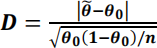
for testing H0: θ = θ0 where θ0 = 0.11.
(ii) Use the value of d determined in (i) and the Normal approximation to the Binomial distribution to determine the approximate p-value for testing H0: θ = 0.11. (A continuity correction is not required.) State your conclusion regarding H0: θ = 0.11 based on the approximate p-value.
(iii) Is the value θ = 0.11 an element of an approximate 95% confidence interval for θ based on the asymptotic Gaussian pivotal quantity? Explain why or why not using only the p-value determined in (ii).
(d) (i) For your data determine the observed value of the likelihood ratio statistic λ(θ0) where θ0 = 0.11.
Note: The following R code will calculate the likelihood ratio statistic for a test of the null hypothesis that theta = theta0 if the maximum likelihood estimate of theta is thetahat and the sample size is n:
lambda<-(-2*log((theta0/thetahat)^(n*thetahat)*((1-theta0)/(1-thetahat))^(n-n*thetahat)))
(ii) Use the value of λ(0.11) and the asymptotic distribution of the likelihood ratio statistic to determine the approximate p-value for testing H0: θ = 0.11. State your conclusion regarding H0: θ = 0.11 based on the approximate p-value.
(iii) Is your conclusion in (ii) the same as your conclusion in (c)(ii)? Briefly explain why you would (or would not) expect these conclusions to be the same.
(iv) Is the value θ = 0.11 an element of a 15% likelihood interval for θ? Explain why or why not without determining the interval.
Problem 2: Tests of hypothesis for Poisson model
The purpose of this problem is to test the hypothesis H0 : θ = θ0 for Poisson(θ) data. See Sections 5.1 to 5.3, and Table 5.2 of the Course Notes.
In this problem you will continue to analyse the Twitter data set that is being used in this course. Make sure you use the same individual data set that you generated, saved, and uploaded to the LEARN Dropbox for Assignments 1 to 3.
All written answers must be in full sentences.
Note: When conducting a test of hypothesis you should use a two-sided test unless otherwise stated. Be sure to explain how the p-value is determined. When stating a conclusion about a null hypothesis please use the guidelines in Table 5.1 of the Course Notes.
In this problem you will examine the data for the variate hashtags (the number of hashtags used in a tweet) for all the data in your data set.
Let the random variable Y be the number of hashtags used in a tweet. Assume that Y has a Poisson(θ) distribution.
(a) The parameter θ corresponds to what attribute of interest in the study population?
(b) What is the maximum likelihood estimate of θ for your data set?
(c) Is the Poisson model a good fit to your data? Justify your answer using numerical and graphical summaries.
Note: Problem 4 on Assignment 3 also involved deciding on how well the Poisson model fit the data.
Twitter recommends using no more than 2 hashtags per
tweet: https://help.twitter.com/en/using-twitter/how-to-use-hashtags You are interested in whether the mean number of hashtags in the study population equals 2.
(d) (i) For your data determine d, the observed value of the test statistic
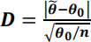
for testing H0: θ = θ0 where θ0 = 2.
(ii) Use the value of d determined in (i) and the Normal approximation to the Poisson distribution to determine the approximate p-value for testing H0: θ = 2. (A continuity correction is not required.) State your conclusion regarding H0: θ = 2 based on the approximate p-value.
(iii) Is the value θ = 2 an element of an approximate 90% confidence interval for θ based on the asymptotic Gaussian pivotal quantity? Explain why or why not using only the p-value determined in (ii).
(e) (i) For your data determine the observed value of the likelihood ratio statistic λ(θ0) where θ0 = 2 for your data.
Note: The following R code will calculate the likelihood ratio statistic for a test of the null hypothesis that theta = theta0 if the maximum likelihood estimate of theta is thetahat and the sample size is n:
lambda<-(-2*log((theta0/thetahat)^(n*thetahat)*exp(n*(thetahat-theta0))))
(ii) Use the value of λ(2) and the asymptotic distribution of the likelihood ratio statistic to determine the approximate p-value for testing H0: θ = 2. State your conclusion regarding H0: θ = 2 based on the approximate p-value.
(iii) Is your conclusion in (ii) the same as your conclusion in (d)(ii)? Briefly explain why you would (or would not) expect these conclusions to be the same.
(iv) Is the value θ = 2 an element of a 10% likelihood interval for θ? Explain why or why not without determining the interval.
Problem 3: Tests of hypothesis for Exponential model
The purpose of this problem is to test the hypothesis H0 : θ = θ0 for Exponential(θ) data. See Sections 5.1 to 5.3, and Table 5.3 of the Course Notes.
In this problem you will continue to analyse the Twitter data set that is being used in this course. Make sure you use the same individual data set that you generated, saved, and uploaded to the LEARN Dropbox for Assignments 1 to 3.
All written answers must be in full sentences.
Note: When conducting a test of hypothesis you should use a two-sided test unless otherwise stated. Be sure to explain how the p-value is determined. When stating a conclusion about a null hypothesis please use the guidelines in Table 5.1 of the Course Notes.
In this problem you will examine the data for the tweet.gap.hour variate excluding tweets which are the first tweets of the day for all the data in your data set. Recall that you analysed the fit of the Exponential model to these data in Problem 5, Assignment 2.
Let the random variable Y be the time between tweets which are not first tweets of the day. Assume that Y has a Exponential(θ) distribution.
(a) The parameter θ corresponds to what attribute of interest in the study population?
(b) What is the maximum likelihood estimate of θ for your data set?
Suppose you have been hired by Twitter to decide whether the mean time between tweets excluding tweets which are not the first tweets of the day number in the study population is 2.5 hours.
(c) (i) For you data determine d, the observed value of the test statistic
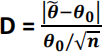
for testing H0: θ = θ0 where θ0 = 2.5.
(ii) Use the value of d determined in (i) and the Normal approximation to the Exponential distribution to determine the approximate p-value for testing H0: θ = 2.5. State your conclusion regarding H0: θ = 2.5 based on the approximate p-value.
(iii) Is the value θ = 2.5 an element of an approximate 99% confidence interval for θ based on the asymptotic Gaussian pivotal quantity? Explain why or why not using only the p-value determined in (ii).
(d) (i) For your data determine the observed value of the likelihood ratio statistic λ(θ0) where θ0 = 2.5.
Note: The following R code will calculate the likelihood ratio statistic for a test of the null hypothesis that theta = theta0 if the maximum likelihood estimate of theta is thetahat and the sample size is n:
lambda<-(-2*log((thetahat/theta0)^n*exp(n*(1-thetahat/theta0))))
(ii) Use the value of λ(2.5) and the asymptotic distribution of the likelihood ratio statistic to determine the approximate p-value for testing H0: θ = 2.5. State your conclusion regarding
H0: θ = 2.5 based on the approximate p-value.
(iii) Is your conclusion in (ii) the same as your conclusion in (c)(ii)? Briefly explain why you would (or would not) expect these conclusions to be the same.
(iv) Is the value θ = 2.5 an element of a 5% likelihood interval for θ? Explain why or why not without determining the interval.
(e) (i) For your data determine d1, the observed value of the test statistic

for testing H0: θ = θ0 where θ0 = 2.5.
(ii) Use the value of d1 determined in (i) and the exact distribution of D1 to determine the p-value for testing H0: θ = 2.5 (see Table 5.3). Use the R command pchisq for your calculation. State your conclusion regarding H0: θ = 2.5 based on the p-value.
(iii) Is your conclusion in (ii) the same as in (d)(ii)? Briefly explain why you would (or would not) expect these conclusions to be the same.
Problem 4: Tests of hypotheses for Gaussian data
The purpose of this problem is to test the hypotheses for Gaussian data. See Sections 5.1 to 5.3, and Table 5.3 of the Course Notes.
In this problem you will continue to analyse the Twitter data set that is being used in this course. Make sure you use the same individual data set that you generated, saved, and uploaded to the LEARN Dropbox for Assignments 1 to 3.
All written answers must be in full sentences.
Note: When conducting a test of hypothesis you should use a two-sided test unless otherwise stated. Be sure to explain how the p-value is determined. When stating a conclusion about a null hypothesis please use the guidelines in Table 5.1 of the Course Notes.
In this problem you will examine the data for the tweet.gap.hour variate for first tweets of the day for which the tweet gap is less than 24 hours for the subset of your data set consisting of tweets from the three personal accounts which you chose. This variate is describing the time between last tweet of the day and first tweet of the next day excluding first tweets which do not happen on the next day. This time might be described as the “downtime” for a user.
Note: This variate can be accessed using the R command
dataset$tweet.gap.hour[dataset$first.tweet == 1 & dataset$tweet.gap.hour < 24]
Let the random variable Y be the gap time in hours for first tweets of the day and for which the tweet gap is less than 24 hours. Assume that Y has a G(μ, σ) distribution.
(a) The parameter μ and σ correspond to what attributes of interest in the study population?
(b) Give the sample mean and sample standard deviation for this variate.
(c) Give the sample skewness and sample kurtosis for this variate.
(d) Give a qqplot for this variate.
(e) Is the Gaussian model a good fit to these data?
According to 2013 data from Statistics Canada (https://www150.statcan.gc.ca/n1/pub/82-003-x/2017009/article/54857-eng.htm) the mean number of hours of sleep for adults aged 18-64 is 7.12 hours with a standard deviation of 2.7 hours. You have been asked to decide whether these values hold for the downtime for tweets in your study population.
(f) Use your data to test the hypothesis H0 : μ = 7.12.
Be sure to state the observed value of the test statistic
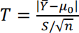
the corresponding p-value, and your conclusion based on this p-value. Explain how the p-value is determined by the R function t.test.
Note: To test hypotheses about the mean for a Gaussian model you can use the R command t.test(). See Chapter 5, Problem 3, for an example. You can also access specific results from using the t.test() command directly. For example, to test the null hypothesis that the mean of a Gaussian distribution is 10 for a sample called y, you use the R command t.test(y, mu = 10)$p.value and R returns the p-value specifically. You can also use $statistic and $parameter in a similar manner.
(g) Is the value μ = 7.12 an element of a 90% confidence interval for μ? Explain why or why not using only the p-value determined in (f).
(h) Use your data to test the hypothesis H0 : σ = 2.7.
Be sure to state the observed value of the test statistic
the corresponding p-value, and your conclusion based on this p-value.
(i) Is the value σ = 2.7 an element of a 99% confidence interval for σ? Explain why or why not using only the p-value determined in (h).
Problem 5: Tests of hypotheses and shiny app
Go to the shiny app: https://shiny.math.uwaterloo.ca/sas/stat231/teststatistics/
You can use this app to explore test statistics and hypothesis tests. You can first choose a probability distribution and a test statistic. You then specify a value for the model parameter under the null hypothesis. You can then adjust the sample size, and set the point estimate of the model parameter resulting from the sample. The right-hand window then displays a plot of the probability distribution corresponding to the test statistic chosen. The plot is then separated into regions based on the value of the resulting test statistic. You should think about how the areas under the probability distribution curves correspond to the resulting p-values.
(a) Binomial(n, θ)
On the shiny app select Binomial as the distribution, Asymptotic Gaussian as the test statistic, 0.1 as the H0 value for θ, and 30 as the sample size. As you move the slider for MLE of θ, you will see how the value of the test statistic and the corresponding p-value for testing H0: θ = 0.1 vary as the value of  varies.
(i) Use the shiny app to complete Table 1 for sample size = 30:
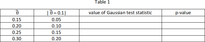
How does the p-value for testing H0: θ = 0.1 change as the quantity | – 0.1| increases? Explain why this behaviour makes sense.
What other value of generates the identical test statistic and p-value as when | – 0.1| = 0.05?
For  = 0.25, use the information from Table 1 to determine what the p-value is for testing H0: θ = 0.1 versus the one-sided alternative hypothesis HA: θ > 0.1.
(ii) On the shiny app select Binomial as the distribution, Asymptotic Gaussian as the test statistic, 0.1 as the H0 value for θ, and 45 as the sample size.
Use the shiny app to complete the Table 2 for sample size = 45.
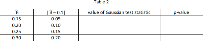
Compare the p-values in Table 2 with the p-values in Table 1. How does the p-value for testing H0: θ = 0.1 change as the sample size increases for a fixed value of | – 0.1|? Explain why this behaviour makes sense.
(iii) On the shiny app select Binomial as the distribution, Likelihood ratio as the test statistic, 0.1 as the H0 value for θ, and 30 as the sample size.
Use the shiny app to complete Table 3 for sample size = 30.
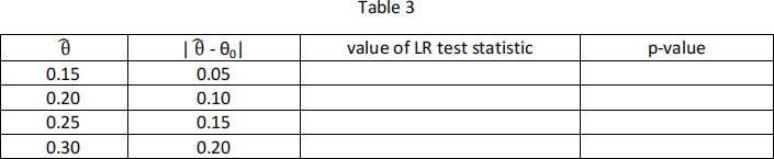
Compare the p-values in Table 3 with the p-values in Table 1. If you use Table 5.1 as your guide for conclusions, is there any value of in Table 1 which gives a different conclusion regarding the hypothesis H0: θ = 0.1 for the same value of in Table 3?
(b) Gaussian mean μ
(i) On the shiny app select G(μ,σ) as the distribution, Mean (μ) as the Test for mean or standard deviation, 0 as the H0 value for μ, and 25 as the sample size, 0.5 as the sample mean, and 2 as the sample standard deviation.
As you change the value of the sample size, you will see how the value of the test statistic and the corresponding p value for testing H0: μ =0 vary as the value of the sample size varies.
Use the shiny app to complete Table 4.
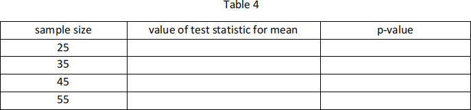
How does the p-value for testing H0: μ =0 change as the sample size increases for a fixed value of the sample standard deviation? Explain why this behaviour makes sense.
(ii) On the shiny app select G(μ,σ) as the distribution, Mean (μ) as the Test for mean or standard deviation, 0 as the H0 value for μ, and 30 as the sample size, 0.5 as the sample mean, and 0.8 as the sample standard deviation.
As you move the slider for sample standard deviation, you will see how the value of the test statistic and the corresponding p-value for testing H0: μ = 0 vary as the value of the sample standard deviation varies.
Use the shiny app to complete Table 5.
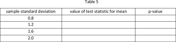
How does the p-value for testing H0: μ =0 change as the sample standard deviation increases for a fixed value of the sample size? Explain why this behaviour makes sense.
(c) Gaussian standard deviation σ
(i) On the shiny app select G(μ,σ) as the distribution, Standard deviation (σ) as the Test for mean or standard deviation, 4 as the H0 value for σ, and 30 as the sample size, 1 as the sample mean, and 4.4 as the sample standard deviation.
As you move the slider for the sample standard deviation, you will see how the value of the test statistic and the corresponding p-value for testing H0: σ = 4 vary as the value of the sample standard deviation varies.
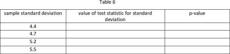
Use the shiny app to complete Table 6.
How does the p-value for testing H0: σ = 4 change as the sample standard deviation increases for a fixed value of the sample mean and the sample size? Explain why this this happens.
(ii) On the shiny app select G(μ,σ) as the distribution, Standard deviation (σ) as the Test for mean or standard deviation, 2 as the H0 value for σ, and 30 as the sample size, 0 as the sample mean, and 2.5 as the sample standard deviation. Record the value of the test statistic and p-value for testing H0: σ = 2.
On the shiny app select G(μ,σ) as the distribution, Standard deviation (σ) as the Test for mean or standard deviation, 4 as the H0 value for σ, and 30 as the sample size, 0 as the sample mean, and 5 as the sample standard deviation. Record the value of the test statistic and p-value for testing H0: σ = 4. Record the value of the test statistic and p-value for testing H0: σ = 4.
What do you notice about the values of the test statistic and p-value for these two cases? Explain why this happens.
(iii) On the shiny app select G(μ,σ) as the distribution, Standard deviation (σ) as the Test for mean or standard deviation, 2 as the H0 value for σ, and 30 as the sample size, -1 as the sample mean, and 2.5 as the sample standard deviation.
As you move the slider for the sample mean, you will see how the value of the test statistic and the corresponding p-value for testing H0: σ = 2 vary as the value of the sample mean varies.
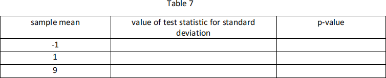
Use the shiny app to complete Table 7.
How does the p-value for testing H0: σ = 2 change as the sample mean increases for a fixed value of the sample standard deviation and the sample size? Explain why this happens.
2021-11-23