MECH203 – Mathematical and Computational Tools for Mechanical Engineers II
Jupyter Notebook Assignment
Optimization
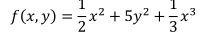
Section A- Find the minimum of the following function:
3) Plot the values of f(x,y)—or log(f(x,y))—x and y at each step during optimization (2 marks).
5) Which method provided the best results, in your opinion? Explain your reasoning (2 marks)
1) Define the function and its analytical gradient in Jupyter notebook. ( 2 marks)
2) Implement a steepest gradient algorithm. Use x 0 = 2, y 0 = 20 as starting points. You can consider that the algorithm has converged to a solution if f(x,y) is within 0.0001 of its optimal value. (4 marks).
4) Use the CG and BFGS algorithms available in the SciPy.optimize.minimize module. Use x 0 = 2,
y 0 = 20 as starting points. (4 marks).
5) How many minima does this function have? (2 marks)
6) Can the computer find them all? (2 marks)
7) Are they local or global? (2 marks)
Section C- Explain in about half-a-page (400 words) how the CG and BFGS algorithms function. Feel free to use equations and graphs. (4 marks)
Optimization
PART 2 – Unconstrained optimization
Let’s practice our coding skills and check if we have a good handle on the basics of local optimization! We’ll do this by writing our own steepest descent solver.Section A- Find the minimum of the following function:
1) Define the function and its analytical gradient in Jupyter notebook. ( 2 marks)
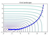
2) Implement a steepest gradient algorithm. Use x 0 = 10, y 0 = 20 as starting points. You can consider that the algorithm has converged to a solution if f(x,y) is within 0.0001 of its optimal value. (8 marks)3) Plot the values of f(x,y)—or log(f(x,y))—x and y at each step during optimization (2 marks).
(PS: this function is positive in all points. You can draw a contour plot with “ax.contour” of the log of this function, which will illustrate that the method is following the gradient. It’s OK if you don’t, you can plot in any way that makes sense to you; but it makes for a cool plot. The advantage of the log is that it makes the x**4 function increase in value less quickly, which facilitates plotting. Note that this example is incomplete: you should insert better labels and legends.)
5) Which method provided the best results, in your opinion? Explain your reasoning (2 marks)
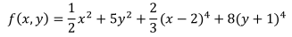
Section B- Minimize the following function instead:
1) Define the function and its analytical gradient in Jupyter notebook. ( 2 marks)
2) Implement a steepest gradient algorithm. Use x 0 = 2, y 0 = 20 as starting points. You can consider that the algorithm has converged to a solution if f(x,y) is within 0.0001 of its optimal value. (4 marks).
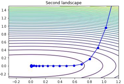
3) BONUS (2 marks): Plot the value of f(x,y), x, and y. For example:
4) Use the CG and BFGS algorithms available in the SciPy.optimize.minimize module. Use x 0 = 2,
y 0 = 20 as starting points. (4 marks).
5) How many minima does this function have? (2 marks)
6) Can the computer find them all? (2 marks)
7) Are they local or global? (2 marks)
Section C- Explain in about half-a-page (400 words) how the CG and BFGS algorithms function. Feel free to use equations and graphs. (4 marks)
2020-02-09