Hello, dear friend, you can consult us at any time if you have any questions, add WeChat: daixieit

Statistics 2: Computer Practical 2

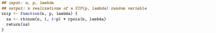
1 Zero-inflated Poisson distribution

1.1 Definition

A zero-inflated Poisson (ZIP) random variable X with statistical parameter  has probability mass function

and f(x; θ)=0 if x  , where  = {0, 1, 2,...} is the set of non-negative integers. Alternatively, X can be defined as X = (1 − B)Z where B and Z are independent random variables with B ~ Bernoulli(p) and Z ~ Poisson(λ).

1.2 What this might be used to model

Imagine that there is a super substance that emits special particles (s-particles) at a particular rate. Non-super substances never emit s-particles. There is also an s-particle detector, which perfectly detects all s-particles emitted in its immediate vicinity.

Two sensible, but statistically quite different, interpretations of ZIP(p, λ) random variables are

1. Z ~ Poisson (λ) is the true but not directly observed random variable of interest. We only are able to observe X which has been randomly set to 0 instead of Z with probability p (independent of Z). For example, Z could model the number of s-particles emitted by a super substance in a given time period, while X models the number detected by an s-particle detector that is perfect in every way except for the fact that we might forget to turn it on. In statistical terminology, we could say that Z is only partially observed.

2. There is no partial observation: X is the true random variable of interest and models counts that are definitely 0 with probability p and otherwise Poisson(λ). For example, X could model the number of s-particles detected by a perfect (and active!) s-particle detector when placed next to a substance, but now the substance might only be super with probability 1 − p.

These differences may seem subtle, and mathematically of course there is no difference in the random variable itself, but the interpretation of the statistical parameters and conclusions about the phenomenon being modelled do differ. Note also the interpretation of a sequence X1,...,Xn of independent ZIP(p, λ) random variables in the examples above:

1. Xi models the number of s-particles detected in the ith round, where for each round we have forgotten to turn on the s-particle detector with probability p, independent of all the other rounds.

2. Xi models the number of s-particles detected in the ith round, where for each round the substance is super with probability 1 − p, independent of all the other rounds (necessarily there should be at least two different substances involved).

In particular, you should realize that this is very different to modelling X1,...,Xn as the number of s-particle detections in n consecutive 1 second intervals by an s-particle detector that is either on or off for all n seconds, or as the number of s-particle detections in n consecutive 1 second intervals when placed next to a single substance that is super with probability 1 − p.

2 Data for the practical

2.1 Gretzky points data

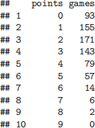
Wayne Gretzky, or “The Great One”, holds a number of National Hockey League (NHL) records as one of the most prolific ice hockey players of all time. We consider here the number of points (goals or assists) he scored in each regular season game the Edmonton Oilers played from 1979–1988 (9 seasons of 80 games each).

In R we can turn this table into a vector containing points scored in each game as follows:

2.2 Bristol City Women’s Football Club goals data

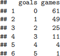
Bristol had a football team in the top tier of domestic football, the Women’s Super League (WSL), from 2011–2015 and from 2017–2021. They were sadly relegated at the end of the 2020-21 season. Although their name has changed during this period, we will refer them as Bristol City Women’s Football Club (BCWFC). We consider here the number of BCWFC goals scored in WSL games since 2011.

As before, we can turn this table into a vector containing goals scored in each game as follows:

3 Questions

3.1 Method of moments estimator

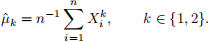
Question 1. [1 mark] Show that the method of moments estimators for p and λ are given by

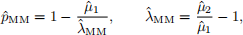
where

Solution

— put your solution here —

Question 2. [1 mark] Compute and report the method of moments estimates for p and λ for both the Gretzky and BCWFC datasets.

I recommend writing a function such as

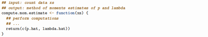
which you can then call on gretzky.data or bcwfc.data to compute the corresponding estimates.

Solution

— put your solution here —

Question 3. [1 mark] Compute and report approximate mean-squared errors for the method of moments estimators of both p and λ (separately), when (n, p, λ) = (100, 0.2, 1.5)

You may find the following function helpful:

Solution

— put your solution here —

3.2 Maximum likelihood estimator

Question 4. [1 mark] The log-likelihood for the ZIP model is

where 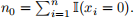The maximum likelihood estimates for (p, λ) do not have a simple expression, so use optim to compute and report the maximum likelihood estimates of p and λ for the Gretzky and BCWFC data.

I recommend writing a function such as

which you can then call on gretzky.data or bcwfc.data to compute the corresponding estimates.

Solution

— put your solution here —

Question 5. [1 mark] Visualize the fitted model by plotting, for each dataset separately, the proportion of games in which x points/goals were scored against x. On each plot, additionally plot the maximum likelihood estimates of these proportions.

Solution

— edit this code, obviously the red dots are not correct —

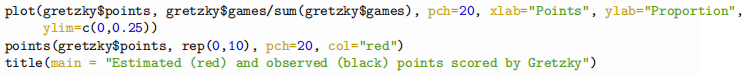
Estimated (red) and observed (black) points scored by Gretzky

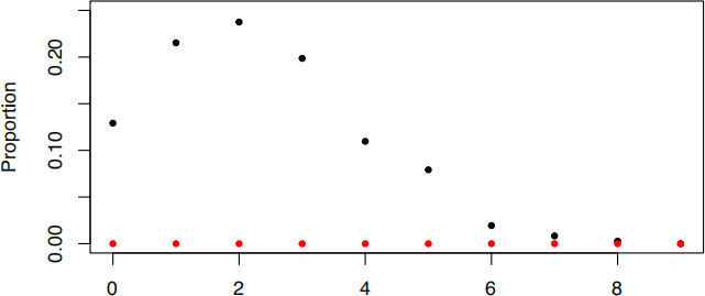
Points

Estimated (red) and observed (black) goals scored by BCWFC

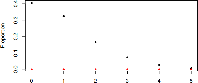
Goals

Question 6. [1 mark] Compute and report approximate mean-squared errors for the maximum likelihood estimators of both p and λ (separately), when (n, p, λ) = (100, 0.2, 1.5)

Solution

— put your solution here —

3.3 Confidence intervals for p and λ

In lectures we have seen that for regular statistical models with a one-dimensional parameter θ, the ML estimator is asymptotically normal with

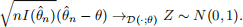
This convergence in distribution justifies the construction of Wald confidence intervals for θ.

In this computer practical, the statistical model is regular but the parameter θ = (p, λ) is two-dimensional.

In this case, the ML estimator is asymptotically (multivariate) normal with

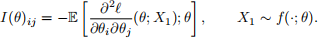
where I(θ) is the 2 × 2 Fisher information matrix whose (i, j)th entries are given by

Note that a random vector Y ~ N (µ, Σ) is multivariate normal if it can be written as Y = µ + AZ, where Z is a random vector of i.i.d. N (0, 1) random variables and Σ = AA^T .

One can deduce from this multivariate asymptotic normality that for i ∈ {1, 2},

where denotes the ith component of  and θi denotes the ith component of θ.

Notice that (I(θ)⁻¹)ii is the ith diagonal entry of the inverse of the Fisher information matrix, and is not in general equal to (I(θ)ii)⁻¹, the inverse of the ith diagonal entry of the Fisher information matrix. In R you can compute numerically the inverse of a matrix using the solve command.

As in the one-dimensional parameter case, when the function θ → (I(θ)⁻¹)ii is continuous, one can replace (I(θ)⁻¹)ii with (I()⁻¹)ii to obtain

The Fisher information matrix for the ZIP model [which you can derive as a separate exercise, but it will take some time] is

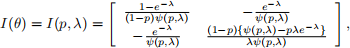
where 

Question 7. [2 marks] Compute and report observed 95% Wald confidence intervals centred at the ML estimate for each of p and λ, and for both the Gretzky and BCWFC data.

To reduce the chance of making mistakes when answering this question and the following question, I recommend writing a function such as

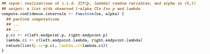
I suggest that you consider writing a few functions that compute important quantities, and call them inside the compute.confidence.intervals function. This can keep the compute.confidence.intervals function from becoming very complicated, prone to bugs and hard to understand.

Solution

— put your solution here —

Question 8. [2 marks] Using simulations, compute and report the approximate coverage of the approximate 1 – α confidence intervals for p and λ used in the previous question, for (–, n, p, λ) = (0.05, 100, 0.2, 1.5).

Solution

— put your solution here —