Hello, dear friend, you can consult us at any time if you have any questions, add WeChat: daixieit

ECMM171P Programming for Engineers

Assignment 3: Projectiles

The path of a projectile is an interesting, important, and sometimes challenging problem. It’s very likely that you will have studied the path of a projectile in the absence of atmospheric drag in basic mechanics, since this can be derived analytically. In the real world, however, drag can significantly alter the trajectory. Unfortunately, in introducing this effect, we lose the ability to analytically obtain solutions for the projectile’s trajectory: simulating the trajectory is therefore required. In this assignment, you will therefore write a Matlab program that computes trajectories under the influence of drag, and use this to solve a simple targeting problem.

1 Theory

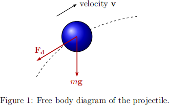
We will neglect any crosswind effects, so that the projectile travels in a two-dimensional plane with coordinates (x, y). The projectile’s position, velocity and acceleration can therefore be rep-resented as vector functions of time, which we denote by r(t)=[rx(t), ry(t)], v(t)=[vx(t), vy(t)] and a(t) respectively. As the projectile travels through space, we will assume that it experiences two forces: acceleration due to gravity, and a drag force Fd acting in the direction opposite to its trajectory. A free body diagram of this scenario can be found in Figure 1. The drag force can be roughly approximated by the drag coefficient cd through the relationship

which also involves the velocity v, air density ρ and the frontal area A (i.e. the two-dimensional cross-section exposed to the drag force). cd is dimensionless and is used to quantify the drag of an object in a fluid: the lower the value, the lower the drag force.

To simulate the trajectory of the projectile, we can use Newton’s second law:

where m is the mass of the projectile and g = (0, g) is acceleration due to gravity with g = 9.81 ms⁻². Since we are interested in the projectile’s trajectory r, we can then utilise the fact that

to give us a ordinary differential equation

Notice that this is a non-linear equation that cannot be solved analytically – we therefore need a computer to simulate it. It is also second-order: that is, it depends on the second derivative of r.

All that is left to do is equip the above with an appropriate set of initial conditions at time t = 0: we will imagine that the projectile is fired from an initial starting height h at an angle of θ degrees and initial speed (velocity magnitude) v0, which gives:

2 Your tasks

Your program will be structured in two parts. In the first part, you will write a function to solve the ODE system defined above. In the second part, you will use these functions to create a simple targeting computer. In all of the below, you should assume that the projectile is a sphere of diameter 0.1 m being fired through air of density ρ = 1.225 kg m⁻³, with corresponding drag coefficient cd = 0.479 and mass m = 5.5 kg.

2.1 Getting a trajectory

In the first part of this assignment, you will write a solver for the ODE in equation (1).

1. Using the techniques discussed in the lectures, first transform equation (1) as a system of first-order equations for the two components of velocity and two components of position, respectively. Mathematically, this system will be expressed as

where y(t)=[vx(t), vy(t), rx(t), ry(t)]. Write a function drag_ode, which takes as ar-guments the time t and the vector y(t), and returns the function F(t, y) as a column vector.

2. Using the lecture notes, write a function called solve_ode_euler, which uses the forward Euler time integration method and your drag_ode function to solve the ODE in equa-tion (1). solve_ode_euler should take as arguments the initial speed v0, the angle of attack θ, the initial height h and a timestep size ∆t. You should also include a maximum integration time as a parameter. You should stop integrating once either the maximum integration time has been reached or once the projectile reaches the ground.

The function should return: the solution time, the two components of v and the two components of r. Include all outputs into a single variable with 5 columns. Each row should contain these values at a given timestep (i.e. the first row is their values at t = 0, the second at t = ∆t, and so on).

3. To validate your implementation, write a function called solve_ode45, which instead uses Matlab’s built-in function ode45 and your drag_ode function to solve the ODE in equation (1). solve_ode45 should take the same arguments and return the same array as solve_ode_euler.

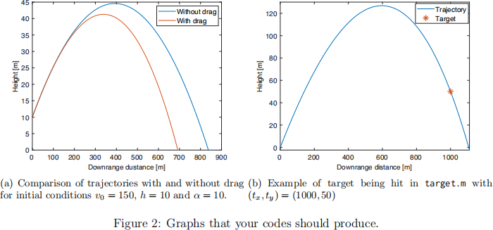
4. You should include a script drag which will prompt the user for initial speed v0, the angle of attack θ, the initial height h and will call the solve_ode_euler function to solve the ODE system and produce a plot that compares this to the analytic solution of the particle trajectory without drag. You may use the following formulae,

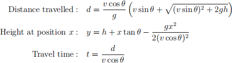
Think carefully about the choice of ∆t. Your script should output a graph that shows the two trajectories with and without drag, as in Figure 2, and will print: initial speed, angle of attack, initial height, travel time, distance travelled and maximum height of the projectile.

2.2 A targeting computer

In your second part, you should use the Matlab’s optimisation package to build a simple tar-geting system. The idea here is that you are given the position (tx, ty) of a target which is downrange from your projectile. Given the constraints that:

● the projectile’s initial velocity can be between 100ms⁻¹ and 800ms⁻¹;

● the projectile’s initial angle can be between 10^◦ and 80^◦.

your program should determine what the initial velocity and angle of the projectile should be in order to hit this target. In all of the below, you can assume that the initial height is h = 0.

1. Write a function called objective, which defines the objective function to be minimised. objective should take as arguments: the two variables being optimised (i.e. the initial velocity and angle), and the target coordinates tx and ty. You may combine the arguments into two variables for convenience. It should call solve_ode45 with the initial conditions and return the shortest distance between the computed trajectory and (tx, ty).

2. Write a function called objective_image. The purpose of this function will be to produce an image, along the same lines as discussed in lectures, that shows the value of the objective function across the range of constraints, as shown in Figure 3. objective_image should take as arguments the target (preferably in a single variable as in objective), and two integers nx and ny, which are the number of pixels to be used to represent the range of initial velocities (in the x-direction of the plot) and the initial angle (in the y-value of the plot). Your function should then plot the objective function across these ranges and produce an output file called objective.pdf.

3. Write a function called target, which takes as two arguments the target’s position tx and ty. Use routines from Matlab’s optimisation toolbox to minimise objective, and return True if the optimisation succeeds, along with v0, θ and the minimum distance; otherwise return False and three zeros.

Some hints:

● This aspect is the most open-ended in the assignment. The function can be quite hard to optimise and is sensitive to initial guesses.

● Use your images from the objective_image as a guide: think about how the opti-misation (minimisation of the objective function) process works and how it might work for some of these images to guide your choices of e.g. initial guesses.

● You can use any combination of functions from the optimisation toolbox, but you may explore fmincon and ga in particular: note the former is much faster than the latter, but is more prone to becoming stuck during optimization.

● You should consider in particular the bounds and args options in these functions and you can consult Matlab’s documentation to determine appropriate arguments to call.

Note that there is no unique solution to this problem: full marks will be awarded for creativity and devising a relatively robust optimisation strategy that works for most cases, which demonstrates knowledge of the programming and numerical techniques under the hood.

4. Finally, write a script called test_target that prompts the user for the coordinates (tx, ty), calls your target function, and prints a message target was hit! along with some

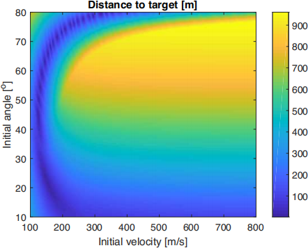
Figure 3: Image of the objective function, which shows the distance between computed tra-jectories and a target (tx, ty) = (1000, 50) for each initial velocity and angle.

information if the target is hit: initial speed, and initial angle. The script should also produce a plot which shows the target and the optimised trajectory, an example of which can be seen in Figure 2(b).

5. On the ELE page, you will find a randomly-generated target to hit for your student ID. You should run your code for this target and submit the objective function image from objective_image along with all your programs.

3 Marking scheme

Your submission will be assessed on the following criteria:

● For the drag part:

– Fully working implementation of the drag_ode function.    [5%]

– Fully working implementation of the solve_ode_euler method.    [20%]

– Fully working implementation of the solve_ode45 method.    [10%]

– Fully working script

   drag and correctly formatted graph.    [10%]

● For the target part:

– Fully working implementation of the objective function.    [5%]

– Fully working implementation of the objective_image function.    [10%]

– Fully working implementation of the target function.    [15%]

– Fully working script test_target which produces correctly formatted graphs of ob-jective function and trajectory.    [10%]

● Discretionary marks for good programming technique, structure and commenting.    [15%]

Details regarding the specific criteria that are used in the above can be found in the module handbook on ELE. You should attempt all of the above routines; incomplete solutions will be given partial credit. Note that these routines will all be marked independently, and you can still receive full credit for complete solutions even if the preceding parts are not fully implemented.

4 Submission

You should package all your files along with the .pdf graph, into a single zip, rar or tar file, and submit using BART.