Hello, dear friend, you can consult us at any time if you have any questions, add WeChat: daixieit

STAT 361 (Fall 2021)

Assignment 4

Guidelines for Preparing Solutions

For questions that needs R coding, please only include the important R output and the necessary results in the main text of your solutions. Present them in a clear and concise fashion (for example, tabulate models and output).

Give descriptions and discussions for your important exploration and findings.

Put long code and output in an Appendix, at the end of EACH problem.

These Appendix sections will NOT be marked, but will be checked as evidence of your in-dependent work.

Prepare your assignment solutions so that it is easy for the readers (in this case, TAs) to follow, without having to search everywhere for your answers from lengthy code and output.

1. Consider Model 2 and Model 3 for the trees data, discussed in Example 5.2.2 and Exam-ple 5.3.1. Suppose a tree has diameter = 8.5 inches and height = 65 feet.

(a) For each model, find a 95% confidence interval for expected volume of the tree, and a 95% prediction interval for the actual tree volume.

(b) For Model 2, carry out an F test of all slopes. Write out the test procedure: hypotheses, test statistics under H0, and your rejection criterion. Is Model 2 useful for explaining tree volume?

Notes: 1) Using R to find all these results are fine, but make sure you know how these intervals and tests are really computed.

2) Recall that if the level 100(1 − α)% confidence interval for θ is defined by P( < θ < ) = 1 − α, then for g(θ) where g() is an increasing function, its confidence interval is defined by P(g() < g(θ) < g()) = 1 − α. Also, what if g() is a decreasing function...

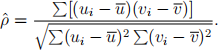
2. The sample correlation coefficient for the observed data u and v is

For a regression model with an intercept and several explanatory variables, show that R² is equal to the square of the sample correlation between the (observed) response vector Y and the vector of fitted values . Please try to complete the proof using vector and matrix notation.

Hints: 1) The response Y =  + r.

2) Define the funny-looking term 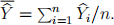 How is it related to

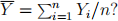
3. Consider the “sale.txt” data posted. A company conducted a survey of a new product to develop a marketing strategy. The response Y is the amount (in thousand dollars) that each individual can spend on the new product. The possible explanatory variable x is the yearly income (in hundred dollars). There are 21 participants in the study.

(a) Fit a simple linear regression for Y and x. Define this model clearly in mathematical form. Assess the model fit by the 3 types of residual plots introduced in Section 5.2. Do you find any problems with the constant variance assumption?

(b) Use the Box-Cox transformation on Y to improve the model. What transformation do you choose? Define a new model in mathematical form based on this transformation. Fit the model, and assess the model performance using suitable residual plot or plots. Is it a good remedy for the problem identified in (a)?

(c) Now consider a model without intercept,

where Yi and xi are the amount individual i can spend on the new product, and his/her yearly income. The error terms are assumed to be i.i.d. N (0, σ² ). Fit this model to the data. Does it fit the data better than the model in (a)? Repeat residual analysis (and plots) for this model as in (a) and comment.

(d) Suppose the true model is

where error terms δi are independent from N (0, σ²xi) distribution. That is, Var(Yi) = Var(δi) = σ²xi. Notice this is a model without an intercept, and for heteroscedastic data! A possible remedy for heteroscedasticity is to consider the model

where In theory, do have equal variances now? Fit this model to the data, and assess the model performance through relevant residual plot or plots. Does it work in fixing the non-constant variance problem for the model in (c)? Remark: Part (d) is really applying a weighted least squares method to the heteroscedastic data. We can also apply it directly to the original data through the lm() function with weights. Try this to see if you get exactly the same output as from the model you fit for (d).

4. The posted file “cars.txt” contains a part of the data collected on fuel consumption and 6 aspects of automobile design and performance for 32 automobiles. The 7 (numeric) variables are given in the following columns.

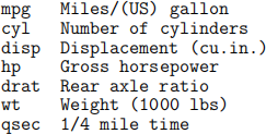
Let miles per gallon be the response variable. Consider all other variables as potential explanatory variables. Build multiple regression models for explaining the miles per gallon variable. Present at least two models that are interesting and appropriate for the data. Assess the model fit based on R² and residual analysis (include some residual plots to support your discussion). In your model explorations, it may be helpful to think intuitively what factors may affect fuel consumption/efficiency of automobiles.