Hello, dear friend, you can consult us at any time if you have any questions, add WeChat: daixieit

Intro to Image Understanding (CSC420)

Assignment 3

General Instructions:

● You are allowed to work directly with one other person to discuss the questions. How-ever, you are still expected to write the solutions/code/report in your own words; i.e. no copying. If you choose to work with someone else, you must indicate this in your assignment submission. For example, on the first line of your report file (after your own name and information, and before starting your answer to Q1), you should have a sentence that says: “In solving the questions in this assignment, I worked together with my classmate [name & student number]. I confirm that I have written the solutions/-code/report in my own words”.

● Your submission should be in the form of an electronic report (PDF), with the answers to the specific questions (each question separately), and a presentation and discussion of your results. For this, please submit a file named report.pdf to MarkUs directly.

● Submit documented codes that you have written to generate your results separately. Please store all of those files in a folder called assignment3, zip the folder and then submit the file assignment3.zip to MarkUs. You should include a README.txt file (inside the folder) which details how to run the submitted codes.

● Do not worry if you realize you made a mistake after submitting your zip file; you can submit multiple times on MarkUs.

Part I: Theoretical Problems (50 marks)

[Question 1] Laplacian of Gaussian (25 marks)

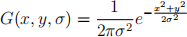
The Laplacian of Gaussian operator is defined as:

where the Gaussian filter G is:

The characteristic scale is defined as the scale that produces the peak value (minimum or maximum) of the Laplacian response.

1. (10 marks) What scale (i.e. what value of σ) maximises the magnitude of the re-sponse of the Laplacian filter to an image of a black circle with diameter D on a white background? Justify your answer.

2. (5 marks) What scale should we use if we want to instead detect a white circle of the same size on a black background?

3. (10 marks) Experimentally find the value of σ that maximizes the magnitude of the re-sponse for a black square of size 100×100 pixels on a sufficiently large white background.

Hint: You can simply implement this task and automatically test for a large set of samples. You may also want to first generate the samples in log-domain to accurately locate the optimal value in a large spectrum.

[Question 2] Corner Detection (25 marks)

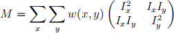
For corner detection, we defined the Second Moment Matrix as follows:

Let’s denote the 2×2 matrix used in the equation by N; i.e.:

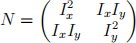
1. (10 marks) Compute the eigenvalues of N denoted by λ1 and λ2?

2. (15 marks) Prove that matrix M is positive semi-definite.

Part II: Implementation Tasks (100 marks)

[Question 3] Local Descriptor: Histogram of oriented gradients (60 marks)

The histogram of oriented gradients (HOG) is a feature descriptor used in computer vision and image processing for the purpose of object detection. The technique counts occurrences of gradient orientation in localized portions of an image. This method is similar to that of scale-invariant feature transform (SIFT) descriptors, and shape contexts (a similar technique we have not seen in class), but differs in the sense that it is computed on a dense grid of uniformly spaced cells and uses overlapping local contrast normalization for improved accuracy. Until deep learning, HOG was one of the long-standing top representations for object detection.

        In this assignment, you will implement a variant of HOG. Given an input image, your algorithm will compute the HOG feature and visualize it as shown in Figure 1 (the line directions are perpendicular to the gradient to show edge alignment).

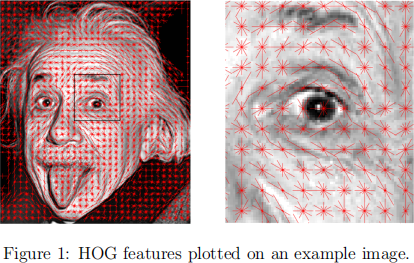
        The orientation and magnitude of the red lines represent the gradient components in a local cell. A HOG descriptor is formed at a specified image location as follows:

1. Compute image gradient magnitudes and directions over the whole image, thresholding small gradient magnitudes to zero. You should empirically set a reasonable value for the threshold for each of the input images.

2. Center a cell grid (m × n) on the image. To create this grid cell, assume the grid cells are square and we have a fixed-size length for each of the cells in this grid; let us call that size τ . For example, if your image size is 1021 ×975 and τ = 8, then you will have a grid size of (m = 127) × (n = 121). You can ignore the boundary of the image that can not be fit into a grid (on either end), i. e., just consider the crop of the image that fits to the grid perfectly, which is 1016 × 968 in this example.

3. For each cell, form an orientation histogram by quantizing the gradient directions and, for each such orientation bin, add the (thresholded) gradient magnitudes. This process can be done in two steps: Imagine gradient orientations are discretized by 6 bins:

Remember is equivalent to where the orientation is not directed. Now cre-ate a 3D array (m × n × 6) where in element (i, j, k) of this 3D array you will store the accumulated gradient magnitudes over all the pixels in the cell (i, j) with gradient orientations corresponding to bin k.

Another approach for constructing the HOG, is to collect the number of occurrences in each bin, rather than accumulating the magnitudes of occurrences; i.e. in element (i, j, k) of the histogram, we store the number of pixels in cell (i, j) with gradient ori-entations corresponding to bin k

Choose reasonable values for the threshold and cell size, and then visualize the resulting 3D arrays (using both approaches) on the given images similar to the quiver plot of Fig-ure 1. Briefly, compare the two approaches by inspecting the visualizations.(15 marks)

Hint: You can use any package/function for creating the visualization in Figure 1. One way to do that is to superimpose 6 quiver plots (one for each bin), generated by quiver function in matplotlib package.

For the remaining tasks, you can use either approaches for constructing HOG. Make sure to explicitly mention your choice in the report.

4. To account for changes in illumination and contrast, the gradient strengths must be locally normalized, which requires grouping the cells together into larger, spatially connected blocks (adjacent cells). Given the histogram of oriented gradients, you apply L2 normalization as follows:

● Build a descriptor for the first block by concatenating the HOG within the block. You can use block size = 2, i.e., 2 × 2 block will contain 2 × 2 × 6 entries that will be concatenated to form one long vector.

● Normalize the descriptor as follows:

where is the element of the vector and  is the normalized histogram. e is the normalization constant to prevent division by zero (e.g., e = 0.001).

● Assign the normalized histogram to the first cell of a new histogram array, i.e. cell (1,1).

● Move to the next block of old histogram array with stride 1 and iterate steps 1-3 above, to compute the next cell of the new histogram array.

The resulting new histogram array will have the size of (m − 1) × (n − 1) × 24. Compute normalized histogram arrays for the provided images, and store them in a single line text file where the data is stored row by row (first row then second row etc.). Submit both your code and the files that are generated by your code. Please note that the file should have the same name as the image (e.g. ‘image.jpg’ → ‘image.txt’). (15 marks)

        In addition to the provided images, use your own camera (e.g. smartphone camera) to capture two images of the same scene, one with flash and one without flash. Convert the images to gray-scale, and down-sample the images if needed to avoid excessive computation overhead.

        First, compute the original HOG arrays for these two images and visualize them similar to Figure 1. (5 marks)

        Second, compute the normalized histogram arrays for each of these two images, and store them in two txt files as instructed earlier. (5 marks)

        Third, by comparing the results, argue why or why not the normalization of HOG may be beneficial. Limit your discussion to a paragraph, containing the main points. You can compare the histograms visually or you may want to define a quantifiable measure to compare the histograms for pair of with-flash/no-flash images. If you choose to visually compare, provide the details of your visualization approach for normalized HOG; alternatively, if you decide to quantitatively compare the histograms, include the function you used and your justification in the report. (20 marks)

[Question 4] Corner Detection (40 marks)

        Download two images (I1 and I2) of the Sandford Fleming Building taken under two different viewing directions:

● https://commons.wikimedia.org/wiki/File:Sandford_Fleming_Building_2011_Toronto.jpg

● https://commons.wikimedia.org/wiki/File:Uoft_SF-01.jpg

1. Calculate the eigenvalues of the Second Moment Matrix (M) for each pixel of I1 and I2.

2. Show the scatter plot of λ1 and λ2 for all the pixels in I1 (5 marks) and the same scatter plot for I2 (5 marks). Each point shown at location (x, y) in the scatter plot, corresponds to a pixel with eigenvalues: λ1 = x and λ2 = y.

3. Based on the scatter plots, pick a threshold for min(λ1, λ2) to detect corners. Illustrate detected corners on each image using the chosen threshold (10 marks).

4. Constructing matrix M involves the choice of a window function w(x, y). Often a Gaussian kernel is used. Repeat steps 1, 2, and 3 above, using a significantly different Gaussian kernel (i.e. a different σ) than the one used before. For example, choose a σ that is significantly larger than the previous one (10 marks). Explain how this choice influenced the corner detection in each of the images (10 marks).