Hello, dear friend, you can consult us at any time if you have any questions, add WeChat: daixieit

ECMT2150 INTERMEDIATE ECONOMETRICS, S2 2021

ASSIGNMENT

Instructions:

● Anonymous marking: Do NOT put your name anywhere on your assignment or in the file name. Identify yourself only by your student number.

● Answer all questions.

● A total of 50 marks are available and marks for each question are indicated throughout.

● The assignment is worth 15% of your final grade for this UoS.

● You will need to use STATA (or another regression software program, but not Excel) to complete this assignment.

Submission Instructions:

● Your assignment MUST be typed and submitted as a single file (i.e. .pdf or .docx) online through the Assignment dropbox. It will be checked using Turnitin for plagiarism.

● You must include your STATA commands/do file as an appendix to your assignment.

● This section should be no more than 4 pages long. It should only show your commands and your output.

● NB: In STATA, if you highlight some of the output in the Results window, then right-click, you can:

● Copy and then paste this into Word or some other word processing software. (In Word, Font Courier New in size 9 works well), or

● Copy as a table or picture. This will capture your commands and output. Then you can paste this table or image into Word or some other word processing software.

Assignment: Multiple Linear Regression, Inference, Heteroskedasticity, Endogeneity and IVs

Information on the datasets

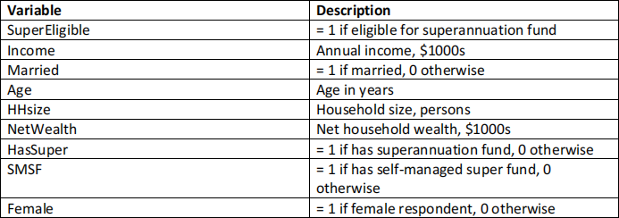
This assignment has two parts and involves applying the econometric techniques developed in the course to two different datasets. Part A will use the dataset ‘retirement.dta’. It contains observations from a sample of the Australian population in 2004 related to their retirement savings plans as well as other social-economic characteristics. See Table 1 for details.

Table 1: Dataset description retirement

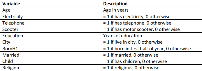
Part B will focus on the dataset ‘fertility.dta’. It includes responses from women in Kenya in 1996. It includes characteristics about whether they have children, their age, number of years of education, and other social-economic status variables about them. See Table 2 for details.

Table 2: Dataset description fertility

Download the two datasets from the ‘Assignment Instructions’ page where you found these instructions. Head to the ‘Assignments’ area on our Canvas site: https://canvas.sydney.edu.au/courses/35741/assignments

Note: there are multiple versions of the two dataset and each student will only have a link to just one. I have edited the two datasets slightly for each version, and by enough that you need to work on your own version. If you work on one of your classmate’s datasets, you will answer one or more questions in the assignment incorrectly and lose marks or be referred to the academic integrity office.

Part A: Retirement [30 marks]

Question 1

a) [2 marks] Investigate the sample properties of the following variables: NetWealth, Income, and Age in the retirement dataset. For each variable, find the mean, standard deviation, minimum and maximum values of its sample distribution. Further, construct a histogram for NetWealth and Income. What do you notice about the histograms you constructed for NetWealth and Income? Include both figures in your typed answer.

b) [1 mark] Estimate the following Linear Probability Model (LPM) using OLS:

Make sure to obtain the usual OLS standard errors (in parentheses) and the heteroskedasticity-robust standard errors (in square brackets). Do you observe any differences between the two versions?

c) [3 marks] Consider the modified version of the White test for heteroskedasticity in which we regress the square of the OLS residuals (i.e. ) on the OLS fitted values (i.e. ) and a square of the OLS fitted values (i.e. ). Explain why the probability limit of the coefficient on should be 1, why the probability limit on the coefficient on should be -1, and why the probability limit of the constant should be 0.

d) [2 marks] For the LPM estimated in b), conduct the modified version of the White test for heteroskedasticity. Confirm that the sample coefficient estimates are reasonably close to the population values described in c).

e) [2 marks] Weighted Least Squares (WLS) is a method for estimating a regression model when the assumption of homoskedasticity does not hold. What must we check when estimating a LPM using WLS?

f) [1 mark] Re-estimate the LPM in b) using WLS. Do you notice any differences compared to the estimates you obtained in b)?

Question 2

a) [1 mark] Estimate the following model using OLS:

Make sure to obtain the usual and robust standard errors (parentheses and square brackets respectively). Is the interaction term significantly different from zero?

b) [3 marks] Re-estimate the model from a) using WLS assuming Var(u | Income) = σ²Income. Compute the usual and robust standard errors (parentheses and square brackets respectively) for the WLS estimator. Is the interaction term statistically significant when using robust standard errors?

c) [1 mark] Consider the WLS coefficient on SuperEligible in b). Is it of any interest by itself? Explain why or why not.

d) [2 marks] Re-estimate the model in b) using WLS again, but this time use the interaction term SuperEligible × (Income − 30). Interpret the coefficient on SuperEligible.

Question 3

a) [1 mark] Estimate the following LPM by OLS:

Report the usual and robust standard errors with your estimation (parentheses and square brackets respectively). Interpret the estimated effect of HasSuper on the probability of having a self-managed super fund.

b) [2 marks] What might be an issue for estimating the ceteris paribus (i.e. all else equal) tradeoff between having a self-managed super fund and being a member of a superannuation fund?

c) [2 marks] The variable SuperEligible is a binary variable equal to 1 if a worker is eligible to join a superannuation fund and 0 otherwise. Discuss what must be satisfied for SuperEligible to be a viable instrumental variable (IV) for HasSuper. How reasonable are these assumptions?

d) [2 marks] Estimate the reduced form model for HasSuper and confirm that SuperEligible is a relevant instrument for HasSuper. As the reduced form model is an LPM, make sure to use robust standard errors.

e) [2 marks] Estimate the structural equation in a) by IV and compare the estimate of β1 with the OLS estimate. Make sure to use robust standard errors when doing this.

f) [3 marks] Test the null hypothesis that HasSuper is exogenous using the Hausman test. Make sure to use a heteroskedasticity-robust test.

Part B: Fertility [20 marks]

Question 1

a) [2 marks] What is the proportion of women with children? What proportion of women live in a city? What is the average age for women and how many years of education do they have on average? Further, construct a histogram for Age and Education. What do you observe about the histograms you constructed for Age and Education? Include both figures in your typed answer.

b) [1 mark] Estimate the following LPM by OLS:

Report the usual and robust standard errors for you estimation results (parentheses and square brackets respectively). Are the robust standard errors very different to the non-robust version?

c) [2 marks] Add the Religion and Married indicator (i.e. dummy) variables to the LPM in b) and test if they are jointly significantly different from zero. What is the robust F-statistic and p-value for this joint test?

d) [3 marks] For the LPM estimated in c), conduct the modified version of the White test for heteroskedasticity. What is the robust F-statistic and p-value for this test? Does the LPM have heteroskedasticity?

e) [2 marks] Is the presence of heteroskedasticity detected in the LPM of practical importance?

Question 2

a) [1 mark] Estimate the following LPM by OLS:

Holding Age fixed, what is the effect of another year of education on the probability of a woman having children? Is the estimate economically significant? Is it statistically significant?

b) [3 marks] The variable BornH1 is an indicator (i.e. dummy) variable equal to 1 if a woman was born during the first half of the calendar year and 0 otherwise. Assuming BornH1 is uncorrelated with the error term for the LPM in a), show that BornH1 is a viable IV candidate for Education.

c) [3 marks] Estimate the LPM from a) using BornH1 as an IV for Education. Contrast the estimated effect of Education with the OLS estimate from a).

d) [3 marks] Include the three binary variables: Electricity, Telephone, and Scooter to the LPM from a). Assuming these three extra regressors are all exogenous, estimate this larger model by OLS and Two-stage Least Squares (2SLS) and compare the estimated coefficients on Education.

Note:

● Include your word count in your document.

● You must type up your answers to this assignment in your own words and submit it through the Assignment dropbox.

● Your typed assignment will be checked using Turnitin for plagiarism.