Hello, dear friend, you can consult us at any time if you have any questions, add WeChat: daixieit

Econ 421: Economic Forecasting and Big Data

Assignment 4

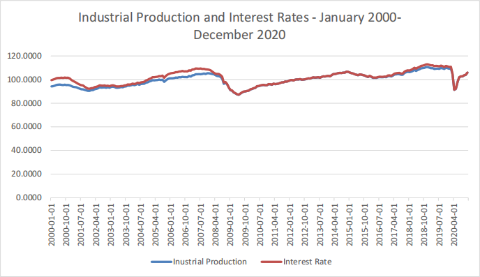
The EXCEL spreadsheet IP_R_trend_assignment4.xlsx contains monthly data on industrial production from January 2000 until December 2020, and on interest rates for the same period.

Additionally, the file contains a time trend variable.

In this assignment you will evaluate the performance of the following models for forecasting the growth rate of industrial production, at forecast horizon h = 1 month ahead.

First, define the target variable to be forecasted as follows:

where IP denotes industrial production. Thus, we have defined y to be the growth rate of IP.

Also, call the interest rate variable R and the deterministic trend variable trend.

Forecasting models to utilize in this assignment

The forecasting models that you will evaluate are the following:

a) Simple Rolling Mean (Moving Average) Model:

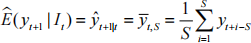
Here, let S=12. Such simple models are good starting points for forecasting.

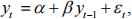
b) Autoregressive Model:

where  and  are constants (i.e., model parameters or coefficients) and is a stochastic disturbance term (i.e., error term). This model is called an autoregressive model of order 1 (i.e., and AR(1) model), and is widely used in many disciplines. Recall that when =1this model is a random walk with drift. The random walk with drift model is widely used as a benchmark model (i.e., a great model against which to compare other forecasting models) when the data are nonstationary. However, you are forecasting the growth rate of industrial production, which is stationary. In such cases, you should expect, when fitting models of the above AR(1) variety that || < 1.

c) Multivariate Model with an Autoregressive Component I:

where , , , and  are constants (i.e., model parameters or coefficients) and is a stochastic disturbance term (i.e., error term). This model is called an autoregressive model of order 1 (i.e., and AR(1) model), and is widely used in many disciplines.

d) Multivariate Model with an Autoregressive Component II:

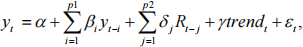
where , , , and  are constants (i.e., model parameters or coefficients) and is a stochastic disturbance term (i.e., error term). This model is called an autoregressive model of order p1 with exogenous variables (the interest rate and trend variables), sometimes known as an ARX(p1) model. This type of model exhibits richer dynamics than the previous models, and variants of it are widely used in many disciplines.

Deliverables for this assignment:

1. Data Visualization:

Create plots of the data series used in the above forecasting models and discuss.

2. Forecasting Exercise:

(1) Construct h=1 step ahead forecasts for the target variable using the four models in a real-time forecasting experiment setup. Namely construct real-time 1-step ahead forecasts for the period 2011:1-2020:12, using the period 2000:1 until 2010:12 as your initial training sample. For models 2 to 4, use a rolling estimation scheme when re-estimating your models prior to each estimation stage. You decide how long to make the rolling window.

Hint: If you are using Excel, the LINEST command can be used for multiple regression. For example, for two explanatory variables the command might look something like LINEST(C2:C21,A2:B21,TRUE,FALSE).

(2) Report forecasts and forecast errors for the 3 models graphically. Additionally include a small table stating the min, max, mean, median, and standard deviation of the forecasts and forecasts errors for each model.

(3) Report mean square forecast errors (MSFE) for the three models. Select the “best” model based on this forecast evaluation criterion.

(4) Repeat (3), but using a different forecast accuracy measure, namely mean absolute forecast deviations (MAFD). Is the “best” model different when you use MAFD instead of MSFE to select amongst the models? Do you think that the use of different forecast accuracy measures might in general lead to a different ranking amongst the models?

(5) Now, using the “best” model selected in (4), create a series of 12 dynamic forecasts for industrial production growth, for the period 2021:1-2021:12. The way to do this is to use earlier forecasts to substitute in for missing future observations, as you “roll” through the ex-ante forecasting period. Report these forecasts. Can you guarantee that these forecasts are MSFE-“better” that those that you would construct if you instead used one of the other models?

Hint: To read about what is meant here, read slides 25-32 in the Eviews tutorial at: https://www.eviews.com/Learning/forecasting.html

Expectations:

Include all calculations and details in your solution to the assignment.