Times Series Analysis and Forecasting Project
Hello, dear friend, you can consult us at any time if you have any questions, add WeChat: daixieit
Times Series Analysis and Forecasting Project
(1) Preamble
• Must be completed in a team of 4 or more students. There will be no exceptions to this rule.
• This project must be submitted in a narrated PowerPoint Presentation format only.
• This project is worth 20%.
• Students are free to use any software of their choice. Please see Software Support.
• Your entire presentation should be less or equal to 40 minutes.
• Help: Contact the TA at: "Annie Shamirian" <[email protected]>
(2) Due Date and what to submit
• This project is due by [April 5, 2024, 11:59 PM]. Please note that late submissions will not be accepted.
• Only one project should be submitted per team. The team leader can make that submission on OWL.
• Please submit One narrated PowerPoint, including results for Part A and Part B.
• Please submit the file to OWL. Submit in a single PowerPoint presentation:
• For how to narrate a PowerPoint, please see: https://support.microsoft.com/en-us/office/record-a-slide-show-with-narration-and-slide-timings-0b9502c6-5f6c-40ae-b1e7-e47d8741161c
• Some points to note:
o Turn off your camera; Only your audio recording is sufficient.
o Do not convert your narration to a video; Upload the file only as PowerPoint.
o Your entire presentation should be less or equal to 40 minutes.
(3) Grading and accountability
• This project is worth 20% of your grade. Your overall effort and accuracy will be used to inform your grade.
▪ ***Your entire presentation should be less or equal to 40 minutes. ***
• On the first page of the report please list:
o What each member did.
o What was each member’s overall contribution to the project (e.g., 10%, 20%, 50%, etc.)
• Take note of the following how your grade for the project will be determined:
Percent Descriptor
90-100 Brilliant. Zero or near errors. There is very strong evidence of complete mastery in the analysis and reporting of the results. If applicable, strong explanation on Zoom.
80-89 Outstanding. Some errors are present, but there is strong evidence of comprehensive understanding in the analysis and reporting of the results. If applicable, strong, outstanding explanation on Zoom
70-79 Very Good. More errors are present, but there is evidence of a very good understanding of the analysis and reporting of the results. If applicable, very good explanation on zoom
60-69 Good. A good effort with weaker evidence of a very good understanding is shown in the analysis, reporting, and explanation of the results. If applicable, good explanation on zoom
50-59 Average.
0-49 No submission/thing piece of work/plagiarism
o Please note your grade will be determined based on your presentation work and, if necessary, your explanation in an interview in person or on Zoom. More weight might be given to the person's presentation. So, if your presentation part is excellent but you cannot explain to the instructor what you did, this will impact your grade. Please note that one or more persons from the group may be chosen for this interview.
• In addition, your contribution to the team will determine your grade. The grade for each team member will be a function of the contribution of each team member using the following equation:

Example 1 Suppose a team with 4 members has contributions of 40%, 30%, 20%, and 10%, respectively.
If the grade earned for the project is 15%, the individual grades will be respectively:
40/40×15 =15%; 30/40×15 = 11.25%; 20/40× 15=7.5%; 10/40× 15 =3.75%
Example 2: Suppose a team with 4 members has contributions of 25%, 25%, 25%, and 25%, respectively.
If the grade for the project is 18%, the individual grades will be respectively:
25/25×18 =18%; 25/25 ×18 = 18%; 25/25× 18=18%; 25/25× 18 =18%
(4) Academic integrity
**WARNING** Any non-compliance with academic integrity may result in a zero grade in the course and a notation on your transcript.
(5) Referencing
• Provide a reference list of sources you used to complete your project. Please use APA style.
Part A:
About ARIMA and VAR
Preamble: Open this link: https://www150.statcan.gc.ca/t1/tbl1/en/tv.action?pid=3610010401
It will take you to Gross domestic product, expenditure-based, Canada, quarterly
Ensure that you have the following customization for the table:
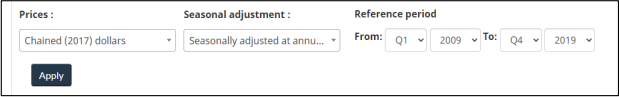
Then Click Apply.
Download data on
• Gross domestic product at market prices
• Final consumption expenditure
• Gross fixed capital formation
Required for the presentation.
(1) Consider the period 2009Q1 to 2019Q4. Convert your data to seasonally adjusted at quarterly rates and produce three individual graphs for the series. Also, produce summary statistics. Discuss your results.
Label your series as follows in your graphs and tables:
GDP = Gross domestic product at market prices
CON = Final consumption expenditure
GFC Gross fixed capital formation
(2) Consider the period 2009Q1 to 2019Q4. Apply the natural logarithm transformation to your series GDP, CON, and GFC. Label them LNGDP, LNCON, and LNGFC, respectively.
(3) Conduct three different unit root tests (e.g., Augmented Dickey-Fuller (ADF) Test, Phillips-Perron (PP) Test, Dickey-Fuller Generalized Least Squares (DF-GLS), Elliott-Rothenberg-Stock (ERS) Point Optimal Test, Zivot-Andrews Test, etc.) on the levels and first differences of your series. Put your results in a table and discuss.
(4) Consider the period 2009Q1 to 2018Q1. Estimate an ARIMA model for LNGDP. Explain your steps and results.
(5) Consider the period 2018Q2 to 2019Q4. Produce a one-step-ahead forecast for LNGDP. Report and explain some forecasting statistics associated with your forecasts.
(6) Consider the period 2009Q1 to 2019Q4. Estimate a VAR using LNGDP, LNCON, and LNGFC. Be sure to apply any required transformations before estimating your VAR. Report and discuss your results.
(7) Explain what Fan Charts are and how they are primarily used.
About Seasonal Adjustment
Preamble. Review: Seasonal Adjustment Packages.
Required for the presentation.
(8) Consider the data here: DATA. Import that province’s retail trade data into an econometric software of your choice. Call this variable retail_RAW
(a) Graph the raw retail trade data for your chosen province. Explain what you observe.
(b) Seasonally adjust the selected retail trade data using any appropriate method. Graph the seasonally adjusted series trend of the series and the irregular component.
(c) Explain how you went about it and provide pertinent statistics demonstrating that your seasonally adjusted series is adequate.
Part B:
Volatility Modelling
Preamble. Open this link: https://www150.statcan.gc.ca/t1/tbl1/en/tv.action?pid=1010012501 and download monthly historical data Standard and Poor's/Toronto Stock Exchange Composite Index, close from January 2011 to February 2020. Call this series TSX.
Required for the presentation.
(9) Apply a first difference natural logarithmic transformations to TSX, and then estimate a conditional volatility model of your choice for the transformed TSX for the period *January 2011 to March 2019*. The more intricate and sophisticated the model, the better. Report your results and explain the steps you took to develop your model and how you know your model is statistically adequate (use diagnostic tests).
(10) Forecast (static) the transformed TSX and its conditional variance over the horizon from February 2019 to February 2020. As applicable, report/graph your results compared to the actual transformed TSX series and the forecasted transformed TSX series. Explain your results and report and discuss forecasting statistics.
About Fractional Integration
Required for the presentation.
(11) What is fractional integration? What are fractional unit root tests?
(12) Explain in detail what ARFIMA models are and when they are used.
2024-04-06