Artificial Intelligence
Hello, dear friend, you can consult us at any time if you have any questions, add WeChat: daixieit
Artiicial Intelligence
You will be examining search strategies for the 15-puzzle, admissible heuristics for a trajectory planning problem, and pruning in alpha-beta search trees. You should submit a report in .pdf format with answers to the questions below.
Question 1: Search Strategies for the 15-Puzzle (2 marks)
For this question you will construct a table showing the number of states expanded when the 15-puzzle is solved, from various start positions, using four diferent search strategies:
(i) Breadth First Search
(ii) Iterative Deepening Search
(iii) Greedy Search (using the Manhattan Distance heuristic)
(iv) A* Search (using the Manhattan Distance heuristic)
Unzip the ile and change directory to path search
unzip path_search. zip
cd path_search
![]() Run the code by typing:
Run the code by typing:
python3 search.py --start 2634-5178-AB0C-9DEF --s bfs
The --start argument speciies the start position, which in this case is:
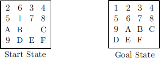
The Goal State is shown on the right. The --s argument speciies the search strategy (bfs for Breadth First Search).
The code should print out the number of expanded nodes (by thousands) as it searches. It should then print a path from the Start State to the Goal State, followed by the number of nodes Generated and Expanded, and the Length and Cost of the path (which are both equal to 12 in this case).
(a) Draw up a table in this format:
|
Start State |
BFS |
IDS |
Greedy |
A* |
||||
|
start1 start2 start3 |
|
|
|
|
|
|
|
|
Run each of the four search strategies from three speciied start positions, using the following combinations of command-line arguments:
Start Positions:
start1: --start 2634-5178-AB0C-9DEF
start2: --start 1034-728B-5D6A-E9FC
start3: --start 5247-61C0-9A83-DEBF
Search Strategies:
BFS: --s bfs
IDS: --s dfs --id
Greedy: --s greedy
A*Search: --s astar
In each case, record in your table the length of the path, and the number of nodes Expanded during the search. Include the completed table in your report.
(b) Briely discuss the efficiency of these four search strategies, with regard to the number of nodes Expanded, and the length of the resulting path.
Question 2: Heuristic Path Search for 15-Puzzle (2 marks)
In this question you will be exploring a search strategy known as Heuristic Path Search, which is a best-irst search using the objective function:
fw (n) = (2 − w)g(n) + wh(n),
where w is a number between 0 and 2. Heuristic Path Search is equivalent to Uniform Cost Search when w = 0, to A* Search when w = 1, and Greedy Search when w = 2. It is Complete for all w between 0 and 2.
(a) Prove that Heuristic Path Search is optimal when 0 ≤ w ≤ 1, assuming
h() is admissible. (You may also assume that A* Search is optimal.)
as m(Hint:)inimizing(show th)afw(t′) i ig(zi) n(g)) (h′(n) o(2)r ( nction(+ wh)(h(n) (n(i) w(th)it(e)h th(sam)e(e) property that h′ (n) ≤ h(n) for all n.
(b) Draw up a table in this format (the top row has been illed in for you):
|
|
start4 |
start5 |
start6 |
|||
|
IDA* Search |
45 |
545120 |
50 |
4178819 |
56 |
169367641 |
|
HPS, w = 1.1 HPS, w = 1.2 HPS, w = 1.3 HPS, w = 1.4 |
|
|
|
|
58 |
13770561 |
Run search.py on each of the three start states shown below, using the Iterative Deepening version of Heuristic Path Search, with w = 1.1, 1.2, 1.3 and 1.4 .
Start Positions:
start4: --start A974-3256-FD8B-EC01
start5: --start 153E-A02C-9FBD-8476
start6: --start 418E-7AD0-9C52-3FB6
Search Strategies:
HPS, w = 1.1: --s heuristic --w 1.1 --id
HPS, w = 1.2: --s heuristic --w 1.2 --id
HPS, w = 1.3: --s heuristic --w 1.3 --id
HPS, w = 1.4: --s heuristic --w 1.4 --id
In each case, record in your table the length of the path, and the number of nodes Expanded during the search. Include the completed table in your report.
(c) Briely discuss how the path Length and the number of Expanded nodes change as the value of w varies between 1.0 (equivalent to IDA*) and 1.4.
Question 3: Graph Paper Grand Prix (5 marks)
We saw in lectures how the Straight-Line-Distance heuristic can be used to ind the shortest-distance path between two points. However, in many robotic applications we wish to minimize not the distance but rather the time taken to traverse the path, by speeding up on the straight bits and avoiding sharp corners.
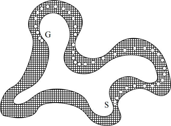
In this question you will be exploring a simpliied version of this problem in the form of a game known as Graph Paper Grand Prix (GPGP).
To play GPGP, you irst need to draw the outline of a racing track on a sheet of graph paper, and choose a start location S = (rS , cS ) as well as a Goal location G = (rG , cG ) where r and c are the row and column. The agent begins at location S, with velocity (0,0). A “state” for the agent consists of a position (r, c) and a velocity (u, v), where r, c, u, v are (positive or negative) integers.
At each time step, the agent has the opportunity to increase or decrease each component of its velocity by one unit, or to keep it the same. In other words,
the(the)n(a)updates(gent mu)sits velo(t choos)ci(e)ty fro(an acc)m(ele) nto(ve) rv )(u(w) ha b+∈b a1nd(0) ,upda(+1}.)te(I)s(t)
its position – using the new velocity – from (r, c) to (r + u′ , c + v′ ). The aim of the game is to travel as fast as possible, but without crashing into any obstacles or running of the edge of the track, and eventually stop at the Goal with velocity (0, 0).
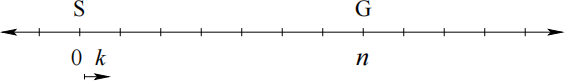
We irst consider a 1-dimensional version of GPGP where the vehicle moves through integer locations on a number line, with no obstacles. Assume the Goal is at location n, and that the agent starts at location 0, with velocity k. We will use M (n, k) to denote the minimum number of time steps required to arrive and stop at the Goal. Clearly M (一n, 一k) = M (n, k) so we only need to compute M (n, k) for k ≥ 0.
(a) Starting with the special case k = 0, compute M (n, 0) for 1 三 n 三 21 by writing down the optimal sequence of actions for all n between 1 and 21. For example, if n = 7 then the optimal sequence is [+ + 。一 。一] so M (7, 0) = 6. (When multiple solutions exist, you should pick the one which goes “fast early” i.e. with all the +’s at the beginning.)
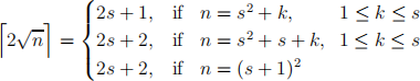
(b) Assume n ≥ 0. By extrapolating patterns in the sequences from part (a),
explain why the general formula for M (n, 0) is
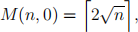
where Lz」denotes z rounded up to the nearest integer.
Hint: Do not try to use recurrence relations. You should instead use this identity:
(c) Assuming the result from part (b), show that if k ≥ 0 and n ≥ 2/1 k(k−1) then
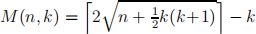
Hint: Consider the path of the agent as part of a larger path.
(d) Derive a formula for M(n, k) in the case where k ≥ 0 and n < 2/1k(k−1).
(e) Write down an admissible heuristic (that approximates the true number of moves as closely as possible) for the original 2-dimensional GPGP game in terms of the function M () derived above.
Hint: Consider the horizontal and vertical motion separately, keeping in mind that, unlike the 15-puzzle, the agent can move in the horizontal and vertical direction simultaneously. Your heuristic should be of this form:
h (r, c, u, v, rG , cG ) = max(M (.., ..), M (.., ..))
Question 4: Game Trees and Pruning (3 marks)
(a) Consider a game tree of depth 4, where each internal node has exactly two children (shown below). Fill in the leaves of this game tree with all of the values from 0 to 15, in such a way that the alpha-beta algorithm prunes as many nodes as possible. Hint: make sure that, at each branch of the tree, all the leaves in the left subtree are preferable to all the leaves in the right subtree (for the player whose turn it is to move).

(b) Trace through the alpha-beta search algorithm on your tree, clearly show- ing which of the original 16 leaves are evaluated.
(c) Now consider another game tree of depth 4, but where each internal node has exactly three children. Assume that the leaves have been assigned in such a way that the alpha-beta algorithm prunes as many nodes as possible. Draw the shape of the pruned tree. How many of the original 81 leaves will be evaluated?
Hint: If you look closely at the pruned tree from part (b) you will see a pattern. Some nodes explore all of their children; other nodes explore only their leftmost child and prune the other children. The path down the extreme left side of the tree is called the line of best play or Principal Variation (PV). Nodes along this path are called PV-nodes. PV-nodes explore all of their children. If we follow a path starting from a PV-node but proceeding through non-PV nodes, we see an alternation between nodes which explore all of their children, and those which explore only one child. By reproducing this pattern for the tree in part (c), you should be able to draw the shape of the pruned tree (without actually assigning values to the leaves or tracing through the alpha-beta algorithm).
(d) What is the time complexity of alpha-beta search, if the best move is always examined irst (at every branch of the tree)? Explain why.
2024-04-02