MAT 338 Spring 2024 Math Application Project #2
Hello, dear friend, you can consult us at any time if you have any questions, add WeChat: daixieit
MAT 338 Spring 2024
Math Application Project #2
Due date: Sun 3/24/2024, 11:59pm
Diving Board Model
This project models a wooden diving board as a Euler-Bernoulli beam, a diferential equation model for how a material bends under stress. We discretize the diferential equation, converting the model into a system of linear equations. As we divide our beam into smaller pieces, our system of equations gets larger. This project will give you an interesting case study of the roles of system size and ill-conditioning in scientiic computation.
Note: As with Project 1, you have no equations to derive for this Project. The mathematical explanation of the equations are included below so you can understand where the model comes from; your assignment is focused on MATLAB programming and related questions. If you wish, you may work with a partner for the entire project. Partners will submit one set of code, one writeup (either separate, or in your live script), and complete one Cover Sheet Google Form.
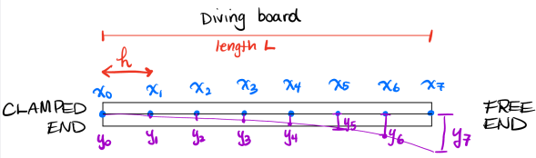
About the model. The vertical displacement of the beamisrepresented by a function y(x), where 0 x L along the beam of length L. We will use SI units in the calculation. The displacement y(x) satisies the Euler-Bernoulli beam equation

where E, the Young’s modulus of the material, and I, the area moment of inertia, are constant along the beam. The right-hand side f (x) is the load applied, including the weight of the beam, in force per unit length.
We have used a simple forward diference formula for the irst derivative, as we’ll derive carefully later this semester. It can be shown that a reasonable approximation for the fourth derivative is this central diference formula

for a small step size h. The discretization error of this approximation is proportional to h2 . We will think of the beam as several consecutive segments, each of length h. Then we will apply the discretized version of the diferential equation on each segment.
Let’s divide the beam into n segments for a positive integer n, and deine h = L/n. Consider the evenly spaced grid 0 = x0 < x1 < . . . < xn = L, where h = xi - xi-1 for i = 1, . . . , n. If we replace the diferential equation (Equation #1) with the diference approximation (Equation #2), we get this system of linear equations for the displacements yi = y(xi ):

Here we develop n equations in the n unknowns y1 , . . . , yn. The coefficient matrix will be deined from the left-hand side of this equation. However, notice that this equation does not take into account any boundary conditions at the ends of the beam we are modeling.
We will model a diving board: a beam with one end clamped at the support, and the opposite end free. This is called a clamped-free beam or sometimes a cantilever beam. In our problem, the boundary conditions for the clamped (left) end and free (right) end are

In particular, notice that these conditions imply that y0 = 0.
But wait! We have a problem. We cannot use Equation 3 to compute y1 , since there is no x-coordinate x-1 . To ix this problem, we introduce a forward diference formula to approximate the fourth derivative at the point x1 near the clamped end. We can use this approximation:

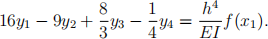
which is valid when y(x0 ) = y' (x0 ) = 0 as we have here. Incorporating Equation 4 into Equation 1 leads us to this equation when i = 1:
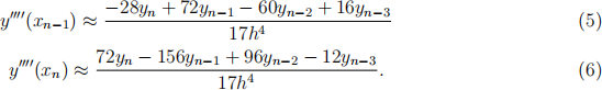
Oh no! Another problem. Similarly, the free end of the beam has no x-coordinates xn+1 or xn+2 . We introduce backward diference formulas to approximate the derivative at xn-1 and xn. Fortunately the approximations below are valid when y'' (xn ) = y''' (xn ) = 0 as we have here.
Now we can write down the system of n equations in n unknowns for the diving board. This matrix equation summarizes our approximate versions of the original diferential equation (1) at each point x1 , . . . , xn , accurate within terms of order h2 :
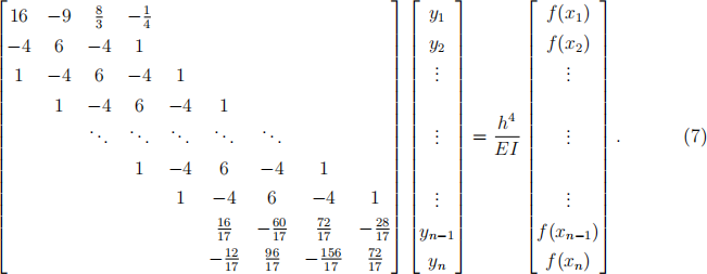
Notice that the matrix A in Equation (7) is a banded matrix, meaning that all entries su伍ciently far from the main diagonal are zero.
Next we choose the parameters for the speciic diving board we will model. Consider a solid diving board composed of Douglas ir, a type of wood with density 480 kg/m3 . Assume the board is L = 2 meters long, 30 cm wide, and 3 cm thick. One Newton of force is 1 kg-m/sec2 , and the Young’s modulus of this wood is approximately E = 1.3 x 10¹⁰ Pascals, or Newton/m2 . The area moment of inertia I around the center of mass of a beam is wd3 /12, where w is the width and d the thickness of the beam. (Make sure you use meters, not cm, in your code.)
Here is the overall approach. You will irst calculate the displacement of the beam with no added weight (i.e., no “payload”), so that f(x) represents only the weight of the beam itself, in units of force per meter. Therefore f(x) is the mass per meter, 480wd, times the downward acceleration of gravity, -g = -9.81 m/sec2 ; that is, the constant f(x) = f = -480wdg. There is an exact theoretical solution of Equation (1) when f is constant, so you can verify your calculation is accurate.
After running your code for the unloaded beam, you will model two further cases. In the irst, a sinusoidal load (or “pile”) will be added to the beam. In this case, there is again a known theoretical solution, but the derivative approximations are not exact. That means you will be able to examine the error of your modeling as a function of the grid size h, and see the efect of conditioning problems for large n. In the second case, you will add a diver on the end of the beam.
Project Programming Activities
1. Write a MATLAB function to deine the coefficient matrix A in Equation (7), which takes as its input the number n of segments along the beam. Then use the MATLAB / command to solve the system for the displacements yi using n = 10 grid steps.
2. Plot the solution from Step 1 against the correct solution
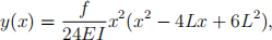
where f = f(x) is the constant deined above. Check the forward error at the end of the beam, x = L meters. (Measure the error in absolute, not relative, terms.) In this simple case the derivative approximations are exact, so your error should be near machine precision.
3. Rerun the calculation in Step 1 for n = 10 · 2k , where k = 1, . . . , 11. Make a table of the absolute errors at x = L and the condition number of A for each n. (Recall that the MATLAB command cond(A,inf) calculates the relative condition number of A, measured in the 1-norm. You may use that value here). For which n is the error smallest? Why does the error begin to increase with n after a certain point? To carry out this step for large k , you may need to ask MATLAB to store the matrix A as a sparse matrix to avoid running out of memory. To do this, just initialize A with the command A=sparse(n,n), and proceed as before.
4. To add a sinusoidal pile to the beam, we add a function of form s(x) = pgsin(L/π x) force term f(x), for constant p. Rerun the calculation as in Step 3 for the sinusoidal load with p = 100 kg/m, making sure to include the weight of the beam itself too. Plot your computed solution against the correct solution,

Answer the same questions as in Step 3, plus this additional question: Is the error at x = L proportional to h2 as claimed in the theoretical derivation above? You may want to plot the error versus h on a log-log graph to investigate this question. Does the condition number come into play?
5. Now remove the sinusoidal load and instead add a 70 kg diver to the beam, balancing on the last 20 cm of the beam. You must add a force per unit length of —g times 70/0.2 kg/m to f(xi ) for all 1.8 xi 2, and solve the problem again with the optimal value of n found in Step #4. Plot the solution and ind the delection of the diving board at the free end.
2024-03-27