Hello, dear friend, you can consult us at any time if you have any questions, add WeChat: daixieit

School of Mathematics and Statistics

Computer Exercise Week 11

STAT3023: Statistical Inference

Semester 2, 2021

Interval estimation of an exponential rate parameter

        Suppose we have a small sample of iid observations from an exponential distribution with unknown rate θ ∈ Θ = (0, ∞). Consider the formal decision problem where the decision space is D = Θ = (0, ∞) and the loss function is L(d|θ) = 1 {|d − θ| > C} for some fixed, known C > 0. In other words, we are interested in forming a fixed-width (of 2C) interval estimate of θ (rather than a “confidence interval”; the main difference is that we are fixing the width, not the coverage probability of the procedure). The risk is the non-coverage probability of this interval; the estimator is the midpoint of the interval.

        We are interested in the risk functions of two “decisions”.

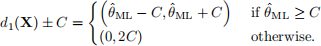
1. An interval based on the maximum likelihood estimator “na¨ıve” interval would simply be  although this would not make complete sense if since then part of the interval would be below zero; we thus modify the interval by defining the centre as

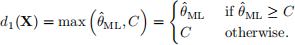
Then the interval estimate is

2. A Bayes procedure for this decision problem using the weight function w(θ) ≡ 1 (the “flat prior”). Since the likelihood is

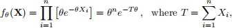
the product of the likelihood and prior/weight function is a multiple of a gamma density with shape n + 1 and rate T; that is, the posterior density is

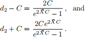
The Bayes estimator is the midpoint of the level set of this density of width 2C; that is,  satisfies

Equivalently,

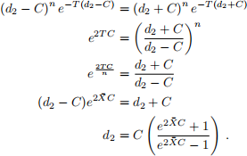
The endpoints of the interval are given by

For simplicity we shall take n = 4 and C = 1.5. We shall make use of the fact that  has a gamma distribution with shape n and rate nθ. We shall firstly approximate the risk functions via simulation, then compute the exact risk functions.

1. (a) Write a function mle.int() that computes the mle-based interval. It should look like

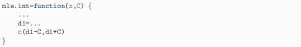
where, of course, the ... parts are replaced with proper R code!

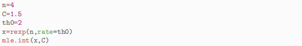
(b) Test it out by generating a test sample:

2. (a) Now write a function bayes.int() which computes the Bayes interval based on the flat prior. It should look like

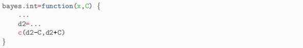
(b) Try it out on your test sample to compare the two intervals.

(c) Visualise the interval by

● plotting the posterior density (using curve());

● adding vertical lines (using lty=2) indicating the interval endpoints;

● adding a horizontal line (using lty=3) at the (common) height of the posterior density at the two interval endpoints;

(see week 10 2(c) for a similar plot). Hint: define m=mean(x), use n and m to define the shape and rate of the posterior (gamma) density, and use curve(...,from=0,to=3/m).

3. Define th=(1:500)/50, L=length(th) and B=1000. Also define

Perform a double loop: at the i-th iteration of the outer loop

● define matrices mle.mat=matrix(0,B,2) and bayes.mat=matrix(0,B,2);

● perform the inner loop: at the j-th iteration of the inner loop

– generate a pseudo-random sample x of size n=4 from an exponential distribution with rate th[i];

– obtain mle-based and Bayes intervals (with C=1.5), saving them in the j-th row of mle.mat and bayes.mat respectively;

● save in the i-th element of noncoverage.mle the number of times the mle-based interval did not cover th[i]; similarly for the Bayes interval in bayes.mat;

Convert the counts in the noncoverage vectors to proportions. Plot (as lines) these proportions against th (red for the mle-based, blue for Bayes). Add an informative heading and legend.

4. The precise form of the risk function for the mle-based interval is different for 0 < θ < 2C and θ ≥ 2C, because for 0 < θ < 2C, the interval can only miss if the mle is too large, whereas for θ ≥ 2C, the interval can miss on both the high side and the low side.

Therefore, for 0 < θ < 2C,

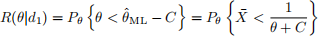
and for θ ≥ 2C,

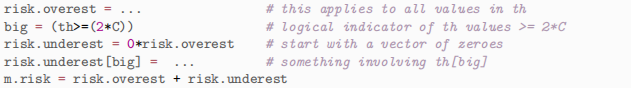
The first probability here is of overestimating, and applies to all values of θ. The second is the probability of underestimating and only applies to θ ≥ 2C.

Since  has a gamma distribution with shape n and rate nθ, we can compute this risk exactly. Compute this risk function for each value in th, save it in a vector called m.risk and plot it against th. Your code should look something like this:

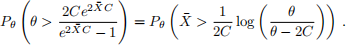
5. The risk of the Bayes interval is given by

The first probability is

Again, because (the Bayes interval’s lower endpoint never drops below zero!), the event in the second probability can only happen for θ ≥ 2C. For such θ it is

Compute this risk function for each value in th (save it in a vector b.risk) and plot it (in blue) against th (you will need to make use of the big indicator and compute risk.overest and risk.underest separately again as you did in the previous question). Add a line plot of the risk of the mle-based interval (in red). Add an informative heading and legend.

6. For which values of th

● does the mle-based interval do better;

● does the Bayes interval do better;

● do the two intervals have similar performance?

Can you describe and explain the behaviour of both curves near θ = 3?