Hello, dear friend, you can consult us at any time if you have any questions, add WeChat: daixieit

Homework 2

ECE 253

Digital Image Processing

Make sure you follow these instructions carefully during submission:

● All problems are to be solved using Python.

● You should avoid using loops in your code unless you are explicitly permitted to do so.

● Submit your homework electronically by following the two steps listed below:

1. Upload a pdf file with your write-up on Gradescope. This should include your answers to each question and relevant code snippet. Make sure the report mentions your full name and PID. You must use the Gradescope page selection tool to indicate the relevant pages of your report for each problem; failure to do so may result in no points. Finally, carefully read and include the following sentences at the top of your report:

Academic Integrity Policy: Integrity of scholarship is essential for an academic community. The University expects that both faculty and students will honor this principle and in so doing protect the validity of University intellectual work. For students, this means that all academic work will be done by the individual to whom it is assigned, without unauthorized aid of any kind.

By including this in my report, I agree to abide by the Academic Integrity Policy mentioned above.

Reports missing any of the above elements may receive no credit.

2. Upload a zip file with all of your scripts and files on Gradescope. Name this file: ECE_253_hw2 lastname_studentid.zip. This should include all files necessary to run your code out of the box.

Problem 1. Adaptive Histogram Equalization (10 points)

        It is often found in image processing and related fields that real world data is unsuitable for direct use. This warrants the inclusion of pre-processing steps before any other operations are performed. An example of this is histogram equalization (HE) and its extension adaptive histogram equalization (AHE).

        The goal of this problem is to implement a function for AHE as described in Chapter 1 of Adaptive Histogram Equalization - A Parallel Implementation1 . The function has the following specifications:

(i) The desired function AHE() takes two inputs: the image im and the contextual region size win_size.

(ii) Using the pseudocode in Algorithm 1 as a reference, compute the enhanced image after AHE.

(iii) You may use loops if necessary. You should not make use of any inbuilt Python functions for AHE or HE.

(iv) The function returns one output: the enhanced image after AHE.

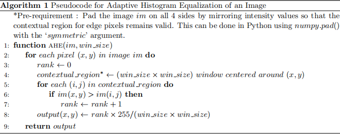
        Evaluate your function on the image beach.png for win size = 33, 65, and 129. In your report, include the original image, the 3 images after AHE, and the image after simple HE (you may use Python inbuilt function for this final HE image only). Make sure to resize all images to ensure they do not take up too much space. Additionally, include your answers (no more than three sentences each) to the following questions:

● How does the original image qualitatively compare to the images after AHE and HE respectively?

● Which strategy (AHE or HE) works best for beach.png and why? Is this true for any image in general?

Problem 2. Binary Morphology (10 points)

In this problem, you will be separating out various objects in binary images using morphology, followed by connected component analysis to gather more information about objects of interest.

(i) For the binary image circles lines.jpg, your aim is to separate out the circles in the image, and calculate certain attributes corresponding to these circles.

● The first step is to remove the lines from the image. This can be achieved by performing the opening operation with an appropriate structuring element. You may find the following functions to be of use.

Python: skimage.morphology.opening()

Feel free to try other functions as well for this question.

● Once we have a binary image with just the circles, the individual regions need to be labeled to represent distinct objects in the image i.e. connected component labeling.

This can be done in

Python using scipy.ndimage.measurements.label().

Feel free to try other functions as well for this question.

● We now have access to individual regions in the image, each of which can be analyzed separately. For each labeled circular region, calculate its centroid and area. Tabulate these values for each connected component. You may use loops for this part of the problem.

Note : This step must be performed entirely by your code without making use of Python’s inbuilt functions (like regionprops()) for connected component analysis. You can still use simple utility functions like sum(), mean(), find() etc.

(ii) In this part, we are interested in performing similar operations on the binary image lines.jpg. Your aim now is to separate out the vertical lines from the horizontal ones in the image, and then calculate certain attributes corresponding to these vertical lines.

● In a similar manner to part (i) above, use the opening operation with a suitable structuring element to remove the horizontal lines in the image.

● Next, perform connected component labeling on the resulting image to identify and label each unique vertical line.

● Finally, for each labeled region, calculate the length (the longer dimension) and the centroid. Tabulate these values for each connected component. You may use loops for this part of the problem.

Note : This step must be performed entirely by your code without making use of Python’s inbuilt functions (like regionprops()) for connected component analysis. You can still use simple utility functions like sum(), mean(), find() etc.

Things to turn in:

● Part (i) & (ii) : The original image, the image after opening, the image after connected component labeling (plot with colorbar), and a table with the desired values for each component.

● The structuring element type and size that was used to perform the opening operation (for both parts).

● Code for the problem.

Problem 3. Lloyd-Max Quantizer (10 points)

For this part of the homework, we study the Lloyd-Max quantizer. Before you get started, carefully study pages 602-603 of the book2 . Then, proceed to implement the following:

(i) Write a function that takes as inputs a greyscale 8-bit (uint8) image, a scalar s ∈ [1, 7] and performs uniform quantization over the entire range [0, 255] so that the output is quantized to an s-bit image. You may use loops for this part if necessary.

(ii) The Python script lloyd python.m is found in the shared homework files. It performs Lloyd Max quantization (optimal quantization in the squared error sense). You can use this function as:

[partition, codebook] = lloyds(training_set, initcodebook)

The input training set is a vector of training data (which is used as an empirical measure of the probability mass function), so you will have to flatten your image (in other words, reshape the image from [M,N] to [M*N, 1].

For the images lena512.tif and diver.tif, calculate the MSE values for s ∈ [1,7] using both your uniform quantizer and the Lloyd-Max quantizer (you may use loops for the Lloyd-Max quantizer as well). Plot the results (MSE versus number of bits). Show one plot for lena512.tif (with both uniform and Lloyd-Max quantization) and another plot for diver.tif. Compare the results for the different quantizers/images and explain them. That is, why does one quantizer outperform the other, and why is the performance gap larger for one image than for the other?

Do not make use of in-built Python functions to calculate the MSE.

(iii) Now use global histogram equalization on lena512.tif and on diver.tif to generate two new images.

Repeat part (ii) for these two new images. Compare them with the previous set of plots. What has happened to the gap in MSE between the two quantization approaches and why?

(iv) Why is the MSE of the 7-bit Lloyd-Max quantizer zero or near zero for the equalized images? One might have thought that equalization is not to the advantage of the Lloyd-Max quantizer, because equalizing the histogram should be flattening the distribution, making it more uniform, which should be to the advantage of the uniform quantizer. Explain this phenomenon.

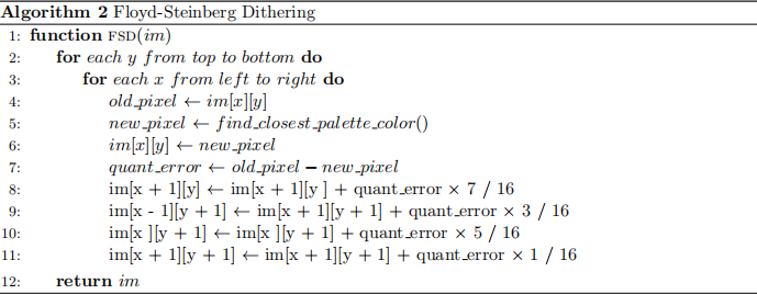
Problem 4. Quantization with Dithering (5 points)

In this problem you will explore the impact of Dithering for image quantization. Specifically, you will be implementing uniform quantization and the algorithm you will be using for dithering is called Floyd-Steinberg.

(i) You will first implement a function that performs uniform quantization with different number of color bands. The function must quantize the image to 10 levels. You can handle each color dimension independently.

(ii) Then you will implement the Floyd-Steinberg shown in algorithm (2) dithering algorithm to study the effects of dithering in each quantized image. The find closest palette color() function simply finds the nearest color value according to 10-level quantization. You can handle each color dimension independently.

        Complete the above two steps on geisel.jpg and answer the questions below. You must include the result of both parts in your report.

1. What differences do you see between the two images?

2. Can you explain what caused these differences?